Economics of Production Lecture

Chapter Summary

Welcome to the next lesson of this module where we will cover the topic of economics of production.

This chapter firstly defines production economics, along with discussing the microeconomics of production, seeking to determine how businesses look to maximise profits, both in the short-term, and the long-term. Following on from this, the chapter explains the Production Possibilities Frontier. Ryanair is used as a case study example throughout the chapter, to demonstrate

Understanding this topic can give a firm a new perspective on their overall management and planning, meanwhile observers can gain an understanding of firm motivations and growth patterns.

Production Economics

Economic theory is to a large extent driven by money - focusing on prices, markets and costs. However, when it comes to production economics, we must also consider the technical production possibility of the business, and how this shapes economic behaviour and the choices involved with production. Production technology in its most general form will consider the relationship between inputs and outputs within a business. Essentially, how well a business can turn its inputs into outputs which can then be sold on, in turn bringing in the relationship of costs and revenue/ profit. The table below showcases how this can be visualised in a table:

Such can also be shown within a graph; displaying how the relationship between inputs and outputs change:

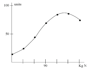
Figure 1 - Relationship between inputs and outputs.

The key takeaway here is that the line is not linear. At the beginning, it could be seen that output increases faster as inputs are increased, seen as efficiency gains, or economies of scale, both which will be discussed later. As inputs increase further, output growth slows, before finally falling. This could be seen as diseconomies of scale, or diminishing returns, again concepts which will be discussed later in more detail.  Essentially, the business can produce at any point on the curve; with its main aim to maximise its own return, and so its profits. It should also be mentioned that the production curve can be any shape depending on the individual business/ market.

However, when considering the production process, it is also important to consider a process whereby there is more than one input. There is then the need to showcase the numerous combinations of inputs which could be used to produce the same output. These are so-called isoquants, shown below:

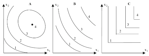
Figure 2 - Production process.

Essentially, each line represents a level of output from the business, which each point on the line a combination of the two inputs which can be used to produce the given level of output. However, each graph showcases a different relationship. For instance, in ‘A’ it could be noted that line 1 shows that it is possible to produce the product/ service with just one output involved, however a combination of the two can also be used. In ‘B’, both inputs are necessary for the output, however there is no maximum, and so this could be thought of as a Cobb-Douglas production function.

Finally, it could be noted that in ‘C’ there is a maximum, with the corners of each line being seen as efficient. With this, it could be seen as a Leontief production function.

Need Help With Your Economics Essay?

If you need assistance with writing a economics essay, our professional essay writing service can provide valuable assistance.

See how our Essay Writing Service can help today!

Economics can be used to recognise the differences between finite resources and infinite wants. Infinite wants can be seen as limitless desires of consumers for goods/ services. However, resources are finite, which in turn will impact on the level of production. For instance, the amount of gold jewellery which can be produced will be dependent on the resources of gold available to be mined. When it comes to production, several factors can be considered, namely:

• Land is where raw materials come from: oil, gas, base metals and other minerals.
• Labour is the ability of individuals to work.
• Capital is production machinery, computers, and office space or retail shops.
• Enterprise is the final factor of production; namely the businesses which bring all the factors mentioned above together to make the final product/ service.

Taking these factors, the Production Possibility Frontier can be constructed (shown below). The graph shows the number of products which can be produced by a business, economy using the finite resources available.

This chapter will discuss the microeconomics of production, seeking to determine how businesses look to maximise profits, both in the short-term, and the long-term.

To start, we must consider the production function of the business; shown below,

Q = f (a, b, c............ n)

Essentially, what we are saying here is that the quantity of output (Q), is determined by the given quantities of output, (a,b,c etc.). Thus, the production function expresses the technological relationship between the quantity of output and the quantities of the various inputs used for the production. Alternatively, it can be changed round to reflect the minimum quantity of each input needed for the final output.

With this, the production function has several assumptions, namely:

1. It is associated with specified period of time.

2. The state of technology is constant during the specified period of time.

3. The producer is expected to use the best and the most efficient technique.

4. The factors of production are divisible.

Production Possibility Frontier

Following on, the Production Possibilities Frontier can be considered. Although, in reality, an economy will produce thousands of goods/ services, for the simplicity of this model it is assumed that the economy can produce two goods. With this, the economy will look to use its factors of production (mentioned above) to produce the two goods, seeking to meet domestic demand. The image below showcases a graphical representation of the frontier:

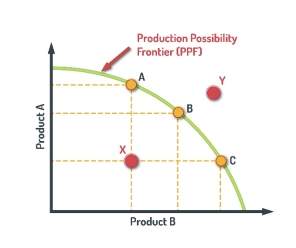
Figure 3 - Production Possibility Frontier

As shown above, several points can be noted on the graph. Points A, B, and C are all on the curve, and so would be seen as efficient, with the economy able to choose production levels for Product A and Product B. Point X would be seen as inefficient given that the economy is producing a combination of goods below its maximum potential. Finally, Point Y would be seen as currently unachievable given that the production is above that of the curve, which as mentioned denotes the maximum production potential of the economy.

Although, the curve can be expanded. For instance, innovation and technological developments allow the economy, and its workforce to become more productive, expanding the production potential of the economy. Furthermore, the size of the workforce could increase, again increasing the productive potential. Considering this, the Solow Growth Model could be considered; a model which suggests that sustainable economic growth can be achieved by two key factors. These are (1) the size of the labour force, and (2) capital, which in turn will consider investments which are designed to increase the productivity of that workforce.

Opportunity Cost and Comparative Advantage

The curve can be drawn at an angle, which in turn will depend on the efficiency at which the economy can produce the good. This then brings into consideration opportunity cost. So, consider two goods, cars and computers. The economy may be more efficient at producing computers. If the economy gave all its resources to cars it could potentially produce a maximum of 1,000 cars, or if it gave all resources to computers it could produce 5,000 computers. This decision may be dependent on specialisation and comparative advantages. For instance, consider a model with Country A and Country B. Assume that both countries have a free-trade agreement (FTA), allowing for the movement of goods between both. Country A may have a comparative advantage in the production of computers, while Country B is specialised, and so more productive in producing cars. The idea here would then be that both countries produce the maximum of the good which they are most efficient at, raising total output. So Country A would solely produce computers, trading them with Country B for cars. A comparative advantage can be defined as ‘the work gains from trade for individuals, firms, or nations that arise from differences in their factor endowments or technological progress’.

Some advantages could be natural; consider Saudi Arabia and crude oil; while others may be developed from education, innovation, or the development of a business cluster. For instance, consider the UK. The development of a financial cluster in London has created an industry which exports £Billions of services each year to international markets. However, at the same time, the UK imports £Billions in manufactured goods from China each year given that it does not have a comparative advantage in low-cost manufacturing.

Cost/ Revenue Equilibrium in Businesses

When it comes to production, a business will seek to supply goods to the market whereby MC=MR; essentially where the marginal cost of producing one extra unit is equal to the marginal revenue earned from producing that one extra good. To understand the basics, a business will make a loss if its costs are higher than its revenue, while it will make a profit if its revenue is higher than its costs. Breakeven will be seen when revenue equals costs; so MC=MR would be seen as the breakeven point for production.

In order to produce goods/ services, generating revenue and profit; a business must employ and purchase scarce inputs which can be seen as factors of production. When it comes to costs, both fixed and variable costs can be discussed. To provide definitions, fixed costs are costs which do not change with production. So, a business paying rent on its factory will remain the same whether it produces 100 units, or 1000 units in the plant. On the other hand, there are variable costs which are seen as costs which move with changes in production. So, materials/ inputs such as electricity and raw materials would be seen as variable costs given that the costs will change as production changes. If the business produces 1000 units they the business will need more raw materials than if it produced 100 units, a variable cost.

With these definitions in mind, it could then be considered that businesses with a high level of fixed costs are able to reduce the total costs per unit by increasing production, known as achieving economies of scale. To provide a definition, economies of scale can be defined as cost advantages that businesses obtain due to their size, output, scale of operation etc., with the costs per unit of output generally decreasing as fixed costs are spread out over more output.

Although, remaining focused on this, the law of diminishing returns can also be considered. This law would suggest that the scale of these cost advantages would decrease as output rises. For instance, assume that after producing 1000 units, the business needed to increase the size of its manufacturing facility to produce more. In this case, fixed costs would then need to rise, reducing the cost advantages associated with economies of scale.

Example - Global Aviation: Ryanair

A good example to mention here would be the case of Ryanair, and how the no-frills airline seeks to benefit from economies of scale to reduce prices. Initially, Ryanair has positioned itself in the aviation industry as a ‘no-frills’ service, selling itself on low prices as opposed to service quality which may be seen in legacy airlines such as BA. However, this model has also allowed Ryanair to maintain healthy profit margins, which as the data below shows is comparable, and even greater than IAG who own British Airways and Iberia.

	Ryanair					IAG (BA/ Iberia)
	2016	2015	2014			2015	2014	2013
Revenue	6,536	5,654	5,037		Revenue	22,858	20,170	18,569
Operating Income	1,460	1,043	659		Operating Income	2,318	1,112	527
Total Assets	11,218	12,185	8,812		Total Assets	28,229	23,652	20,777
Net Income	1,559	867	523		Net Income	1,495	982	126
Shareholder Equity	3,597	4,035	3,286		Shareholder Equity	5,226	3,485	3,909
Current Assets	4,822	5,742	3,444		Current Assets	9,089	7,427	6,018
Current Liabilities	3,370	3,346	2,275		Current Liabilities	11,366	9,801	8,317
ROE	0.43	0.21	0.16		ROE	0.29	0.28	0.03
ROA	0.14	0.07	0.06		ROA	0.05	0.04	0.01
Operating Profit Margin	0.22	0.18	0.13		Operating Profit Margin	0.10	0.06	0.03
Current Ratio	1.43	1.72	1.51		Current Ratio	0.80	0.76	0.72
Asset Utilisation	0.58	0.46	0.57		Asset Utilisation	0.81	0.85	0.89
	Ryanair					IAG (BA/ Iberia)
Capital Structure	2015	2014	2013		Capital Structure	2015	2014	2013
Shareholder Equity	3,597	4,035	3,286		Shareholder Equity	5,226	3,485	3,909
Debt	4,023	4,432	3,084		Debt	8,630	6,617	5,122

One concept here is economies of scale. For airlines, their services have fixed capacity, while most costs are fixed. For instance, a flight from London-Paris will have fixed capacity in terms of 150 seats. To add, most costs, such as staffing, fuel will be fixed; it would be the same if the plane is 50% full or 100% full. Taking this, consider that the highlighted flight has total costs of £5,000. For BA, the flight may be 60% full, so 90 people, meaning that the cost per passenger would be £55.56. However, Ryanair, potentially taking advantage of the elasticity of demand for air travel reduce their prices, attracting more customers and filling 90% of their plane, so 135 passengers. In this case, the costs per passenger will fall to £37.03. Essentially, Ryanair can offer a lower priced product, however still make a similar, or even greater profit margin than BA.

Marginal and Average Costs

For any business seeking to decide on production, two main questions can be asked. The first would refer to the average cost of producing one unit of the good/ service, while the second will consider the marginal cost which will be occurred from producing one more of that good. Initially, it could be considered that the marginal costs of an extra unit may be low, especially if the business has spare capacity in the production process. So, if production was increased, the business could utilise this spare capacity, benefitting from economies of scale and keeping the marginal cost low, representative of the variable costs of production, variable costs which could then be helped by cost savings associated with efficiency and bulk buying of raw materials. However, as this spare capacity is eroded, then the marginal cost may increase. For instance, there could be longer waiting times to use equipment, or the need to hire more staff, making the marginal cost of increasing output by one expensive.

Considering the above, the average cost curve is U-Shaped. Initially, a business can reduce the average cost by increasing production, benefitting from economies of scale, however this is only applicable up to a point. As production increases, the business can then suffer from diseconomies of scale, leading to the average cost rising, which could be brought about by the business needing to expand, i.e. larger factory, more employees. A graph is shown below which plots both the marginal, and average costs.

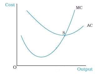
Figure 4 - Marginal and Average Costs

As shown, the point at which the MC curve and AC curve cross is the minimum for average costs. As mentioned above, a business will maximise their own production to a point when MC = MR, shown below in graphical form:

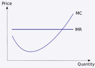
Figure 5 - MC = MR; Business will maximise their own production at the point where MC = MR.

Elasticity of Demand

Considering the example above, it is interesting to consider the elasticity of demand when it comes to production. For instance, in the case of Ryanair, the airline was able to increase demand for its products by reducing the price; allowing it in turn to reduce costs. However, this may not be the case for all goods/ services. For instance, air travel could be considered as an elastic good, one whereby the % change in demand for the good will be greater than the % change in price. On the other hand, an inelastic good is one where the % change in demand would be lower than the % change in price. While an inelastic good may benefit businesses when the price increases, i.e. petrol; cutting prices may not necessarily generate much higher demand.

This can be noted in the petrol market given recent increases in the price. Given that petrol could also be seen as an essential good for consumers/ businesses, the price becomes somewhat irrelevant in the short-term. To visualise this, consider that you have a car, using it to travel to/ from work each day, using 20L of petrol per week. If the price increased, you still need to get to/from work and so your demand for petrol will remain the same, at least in the short-term anyway. When we consider the long-term, the inelasticity of some goods can fall. For instance, if the price of petrol remained high, you could consider alternatives such as public transport/ a bike/ or walking; OR you may consider purchasing a smaller vehicle, or a more fuel-efficient vehicle which will reduce your demand for petrol.

Moving back to the elastic good, a consumer may deem it unessential. So, in the case of air travel, the consumer may (1) forgo the good entirely, or (2) search for an alternative good. To provide an example, consider that you are looking to book a holiday, however the price of the flight you were considering increased by 20%. You may decide that the holiday you were considering is too much, simply not having a holiday; or you may decide to holiday in the UK instead, having a ‘Staycation’ which means you can consider alternative transport such as trains. Furthermore, it could also be considered that the consumer may simply choose a substitute. This will differ by the good/ service; for instance, if the flight above is being provided by BA, a consumer could simply consider a flight by Ryanair as a substitute. Prices will differ between businesses given the competitive nature of the market. This may differ in markets such as petrol given that the good being provided is homogenous. 

Short-Run Costs/ Revenue

In the short-run the business will look to maximise profits; be it where total revenue is greater than total costs.

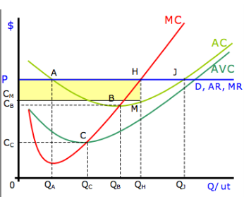
The graph below represents a single firm in a perfectly competitive market. You can tell it is a perfectly competitive market in this example with the demand curve, shown as being perfectly elastic, suggesting that the business can supply as much of the good/ service to the market at the price point ‘P’ (displayed below):

As mentioned above, the MC curve initially falls before rising. In the short-term, the business will look to produce at QH, where the MC line crosses the price line; essentially where MC = MR. However, at this price point, the business can make profits shown by the shaded area, given that the MC crosses the average cost line (here AC) at point B. Points A and J show the breakeven points, suggesting two points at which the business can produce and breakeven. Although, as shown by the shaded area, the business is earning above normal profits at point H, known as abnormal profits. Considering this in a perfectly competitive market, the long-run argument would be that new businesses enter the market, increasing total output and pushing the price lower. However, this argument will differ when other market structures come into play, discussed in another chapter.

Other Costs - Opportunity Costs

When analysing a business’s behaviour, it is important that all opportunity costs of protection are considered. Some of the opportunity costs, such as the wages the business pays to workers are classed as explicit. An explicit cost is defined as a direct payment made to others during running a business; i.e. wages, rent, materials. Other costs, such as the opportunity cost associated with the wages the businesses owner gives up by not taking another job are classed as implicit. Implicit costs are defined as those which have an opportunity cost however there is no payment made, or no asset held. Economic profits will consider both the explicit/ implicit costs into account, while the accounting profit only considers the explicit costs.

Marginal cost

To provide a definition, the marginal cost could be seen as the change in total cost that arises when the quantity produced is increased by an increment of one. So, if the business currently produced 100 units with total costs of £1,000; and increasing this to 101 increased total costs to £1,008 then the marginal cost would be £8. This in turn will impact on revenue, and profit. For example, consider that the business sold each unit for £15, then the total revenue would increase by £15, and the profit would increase by a further £7. So, in this example it is beneficial for the business to increase production as it increases profit. Furthermore, the marginal revenue (MR) is greater than the marginal cost (MC).

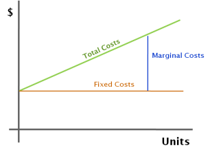
Figure 6 - Visualisation of marginal costs

While marginal revenue can remain constant over a certain level of output, it follows the law of diminishing returns and will eventually slow down, as the output level increases. Perfectly competitive firms continue producing output until marginal revenue equals marginal cost. However, take a business in a less competitive market. They may currently produce 100 units with a profit mark-up of 20%. However, as production is increased, and supply onto the market is increased; if this is not replicated by a rise in demand then the market could become oversupplied; pushing businesses to cut prices to entice more demand. In this case, there is a diminishing return of MR.

Long-Run Costs/ Revenue

When it comes to the long-run, new variables must be considered in terms of production. For instance, costs could increase which are out of the control of the business. Again, consider the airline industry and Ryanair’s business model. In the short term (<1 year), Ryanair can control its costs, be it signing purchase agreements for aviation fuel, setting airport fee’s or offering its employee’s a set wage rate. However, in the long-run, these costs can become variable. For instance, crude oil prices move daily on global markets; meaning that businesses may see a different price when it comes to re-negotiating contracts. So, the price being paid by Ryanair for fuel would vary between 2016 and 2013 given the major differences in oil prices. Furthermore, wages could be impacted on by increases the minimum wages, or be negotiations from trade unions. Finally, airport fee’s and other costs may increase for the airline given changes in the supply chain, and inflationary pressures. Ultimately, what is being mentioned here is that long-run costs are more variable to change; even fixed costs. For instance, a landlord may put up the rent on the buildings rented by the business.

With this, revenues and profits can be affected, especially when the market is also considered. Ryanair operates in a highly competitive marketplace whereby new entrants are adding more capacity into the market, leading to lower prices. If Ryanair increased prices to compensate for higher costs, then it may suffer from a drop-in demand as consumers look elsewhere. This is when economies of scale become important. As mentioned above, business may seek economies of scale through increasing production, allowing them to cut the cost per unit. If this is possible, then Ryanair could maintain its profit margin even while cutting its own prices to remain competitive in the marketplace.

Need Help With Your Economics Essay?

If you need assistance with writing a economics essay, our professional essay writing service can provide valuable assistance.

See how our Essay Writing Service can help today!

The Relationship of LR and SR costs

For many businesses, the division between fixed, and variable costs will depend on the time horizon. So, in the short-term, Ryanair may have fuel as a fixed cost given that they have a purchase contract in place which fixes the price. However, in the long-term, (>1 Year), the contract may expire, in turn making fuel costs variable. To provide another example consider automaker Toyota. Over the short-term it cannot easily expand its production through the opening of new factories; this is a long-term solution. So, in the short-term, it may increase production through hiring more workers for its current factories, in turn focusing on the productivity of current assets. By contrast, over a period of several years, Toyota could build new factories, or close older ones, changing the cost structure.

With this in mind we consider the long-run average cost curve (LRAC) along with the short-run average cost curve (SRAC).

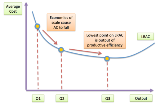
Considering the graph above we can consider the following points:

• The long run average cost curve (LRAC) is known as the ‘envelope curve’ and is drawn on the assumption of there being an infinite number of plant sizes
• Points of tangency between the LRAC and SRAC curves do not occur at the minimum points of the SRAC curves except at the point where the minimum efficient scale (MES) is achieved. This is shown in the graph below. To provide a definition, the MES is seen as the lowest point at which the plant can produce such that its long-run average costs are minimised.
• If LRAC is falling when output is increasing, then the firm is experiencing economies of scale. For example, a doubling of factor inputs might lead to a more than doubling of output.
• Conversely, When LRAC eventually starts to rise then the firm experiences diseconomies of scale, and, If LRAC is constant, then the firm is experiencing constant returns to scale
• The working assumption is that a business will choose the least-cost method of production in the long run.

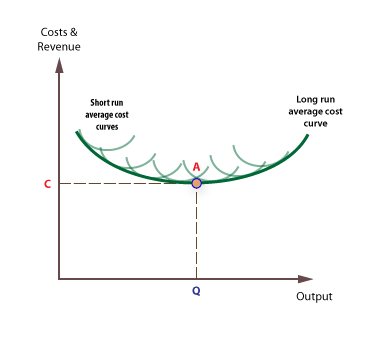
The graph above displays this relationship. SRAC’s are less changeable, leading to multiple curves. Point A would be the equilibrium here, the MES given that it is at the point which minimises the LRAC’s.

The key takeaway here is:

• In the short-run, some inputs are variable, while some are fixed. New firms do not enter the industry, and existing firms do not exit.
• In the long-run, all inputs are variable, and firms can enter and exit the marketplace.

Profit maximisation

Following on from the discussions above, profit maximisation can be seen when the business determines the best output level and price. As noted in the supply/ demand diagram, demand for a product will generally increase as the price of that product falls. From a consumer perspective, this will be support by consumer utility of the products compared with its price. However, by cutting the price when costs are constant, the idea would be that profit would suffer. Although, this may not necessarily be the case. For instance, when we consider the idea of elastic and inelastic demand, it could be considered that a fall in price may drive a much higher increase in demand, considering elastic demand. Furthermore, it could also be considered that as the business increases supply to meet demand, economies of scale can be realised, helping the business to decrease the costs per unit, maintaining profitability; mentioned above in the airline example.

Price Per Unit (AR) (£)	Demand / Output (units)	Total Revenue (TR) (£)	Marginal Revenue (MR) (£)	Total Cost (TC) (£)	Marginal Cost (MC) (£)	Profit (£)
50	33	1650		2000		-350
48	39	1872	37	2120	20	-248
46	45	2070	33	2222	17	-152
44	51	2244	29	2312	15	-68
42	57	2394	25	2384	12	10
40	63	2520	21	2444	10	76
38	69	2622	17	2480	6	142
36	75	2700	13	2534	9	166
34	81	2754	9	2612	13	142

However, when it comes to discussing these concepts we also need to consider the short-term and the long-term. For instance, in the short-term the business may be able to maximise their profits by reducing the price, and benefitting from higher levels of demand (considering the table above). Such a move could also be considered strategic, and may be designed to remove competition from the marketplace and gain market share. In the long-term, businesses may increase their spending on innovation to increase productivity and reduce their own costs. With this, the total supply onto the market may increase, reducing prices further and putting pressure on profits.

Example - Global Oil Markets

A current example of this can be seen within the global oil market. Oil prices fell in 2014/2015 on the back of oversupply in the global market, driven by a rise in non-OPEC supply, growth, and slowing demand growth in the emerging markets. For many producers, this created a situation where the market price of oil was below the current production costs. Considering this with economic theory, the idea would be that these businesses would cut production, rebalancing the market and seeing the price rise back up to an equilibrium point. However, this did not happen for several reasons, being:

1. Oil projects are long-term developments, with businesses committing $Millions, even $Billions to their development. With this, a project may have been approved, and commenced while prices were much higher. Deferring a project, or reducing production from a newly started oil-well could be costlier for the business, and so production will be maintained even if prices are lower than costs. Businesses would hope that prices/ costs can change in the long-term.
2. Many producers have responded to lower prices by increasing production, seeking to increase their own production to reduce the average cost per unit of output. This has been noted in the U.S., whereby Shale Oil producers have increased production, and reduced their prices, making it harder for prices to rise, and supply to fall. A similar situation was also noted in the global iron ore market, whereby the main players of Rio Tinto, BHP Billiton and Vale all continued to increase production in the face of lower prices given that they could decrease their costs.
3. Such moves are strategic in terms of market share, dependant on the market structure. For instance, some businesses may look to maintain current production, even if it is losing money given their hope that competitors may exit the market before them, giving them a stronger market position in the long-run.
4. Technology also plays an interesting point in production, as it provides the innovation needed to reduce costs beyond that of economies of scale. For instance, focusing on the oil industry, better recover rates from improved technology allows producers to decrease costs. Another topical example could be seen within renewable energy, and the decreases seen in costs for offshore wind, making developments more profitable for businesses.

The key takeaway here is that while the economic theory presented above would suggest that a business will look to maximise profits with production.

Key Points

To summarise the chapter, the main points to note are:

• The main goal of the business is to maximise its profits, which will be calculated by total revenue minus total costs.
• When analysing a business’s behaviour, it is important that all opportunity costs of protection are considered. As mentioned in the chapter, some of the opportunity costs, such as the wages the business pays to workers are classed as explicit. Other costs, such as the opportunity cost associated with the wages the businesses owner gives up by not taking another job are classed as implicit. Economic profits will consider both the explicit/ implicit costs into account, while the accounting profit only considers the explicit costs.
• The costs of the business will be reflective of its production process. So, as noted in the chapter, you will notice a relationship whereby the businesses production function gets flatter as the quantity of output increases, also noted as the diminishing marginal product. When it comes to the costs, economies of scale are potentially seen as the business increases output, dependent on the make-up of costs, be it fixed, variable etc.
• However, there would be diminishing returns here; optimal production in the business will be reached when the marginal costs of production equal the marginal revenue.
• A businesses costs can be divided into fixed costs and variable costs. Fixed costs are costs which do not change with output, i.e. rent on current premises; while variable costs do change along with output, i.e. material costs. Although, as we have mentioned, this can change dependant on the time horizon considered. For instance, a cost could be fixed in the short-run given that business decisions are also fixed, however it could become variable in the long-run due to the time available to the business to change. For instance, a business may be fixed in the short-run in terms of the factories it rents, making rental costs fixed. However, in the long-run, the business may have the potential to lease extra space for production, seeing rental costs increase.
• For a business’s total costs, two measures of costs are derived. The first, Average Total Costs considers the average cost, simply the total costs divided by the quantity of output. Marginal cost is the amount by which the total cost will increase if the level of output is increased by 1.
• When it comes to behaviour of businesses in terms of production, it is interesting to consider both marginal costs and average costs. For a typical business, the marginal cost will increase as output increases. However, Average Total Costs should fall at first, signalling economies of scale and efficiency, however should then start to rise as output increases further, known as diseconomies of scale. The marginal cost curve will always cross the average total cost curve at the minimum of the average cost curve.

Practical Chapter

The following chapter will seek to increase your understanding of the economics behind production; and how businesses make their decision on how much to produce.

To start, we must consider the production function of the business; shown below,

Q = f (a, b, c............ n)

Essentially suggesting that the production of the good is a function of the inputs, in this case, a,b,c etc.

Economically, this comes down to profit maximisation. To start, the ability to make a profit will be based on the ability to produce, which can be illustrated by the Production Possibility Frontier, showing the capabilities available to an economy in terms of producing two goods. While the curve may be fixed within the short-run, there is the potential for the curve to be expanded in the long-run through the implementation of new technology/ capital to increase productivity, or through the expansion of the labour force; factors which are both mentioned within Solow’s Growth Model.

Production can simply be seen as an input/ output model, shown below in the figures:

Ultimately, the business here is able to increase production of cereal by increasing the input of nitrogen. Since the curve above is not linear, there is the expectation that the relationship between inputs and outputs is not constant. This brings into discussion the concept of diminishing returns. For instance, if we consider the table above, we can see that increasing the amount of nitrogen used from 60 to 90 brings about a 25-unit increase in cereal production, from 45 to 70. However, increasing the use of nitrogen further, another 30KG increase to 120 only brings about a 15-unit increase in cereal production.

As well as benefits to production, this can also have cost implications, which are known as economies of scale. Economies of scale can be defined as cost advantages that businesses obtain due to size, output, or scale of operation, with cost per unit of output generally decreasing with increasing scale as fixed costs are spread out over more units of output. On the opposite end, we have diseconomies of scale which are seen when increasing output further actually increases the costs per unit.

So, a business will look to maximise its production at a level whereby economies of scale are maximised, benefitting on the cost side. This can be seen in the graph below:

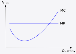
Ultimately, the business will look to produce at a point where MC=MR, and so the marginal cost of producing one extra good is the same as the marginal revenue which will be gained from producing one extra good. Marginal costs can be depicted below, essentially being the change in variable costs as output is increased, although fixed costs can also change in the long-run.

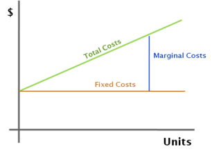
Ultimately, the main point to remember is that a business will look to maximise its profits, and so will change production depending on the costs, prices and market.