Income and Expenditure Lecture

This chapter will consider Income and Expenditure. To provide an overview, the chapter will first consider the circular flow of money through the economy, before discussing demand, as well as income through the IS-LM model. Through all of this it is important that we remember the simple production function as it provides us with a basic understanding of aggregate demand, and the factors which influence it. The simple production function states that output (Q) is a function (f) of:  (is determined by) the factor inputs, land (L), labour (La), and capital (K), i.e.

Q = f (L, La, K)

1.0 Circular flow of Income Model

The visual below provides a basic view of the circular flow of money within an economy:

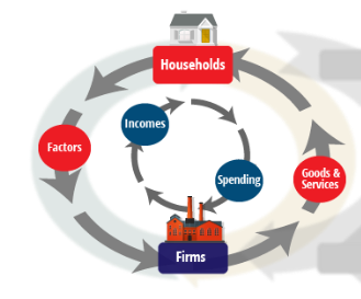
Essentially, in this case there are two actors, namely the ‘households’ and the ‘firms’. The firms supply income to the households in exchange for labour hours worked, while the households then complete the circle by spending their wages in the economy and sending spending income back into the firms. This is the ‘basic’ form of the model as it considers an unbroken loop, however at the same time it does not include potential linkages from the circle which will now be discussed.

To start, consider the consumption function which suggests that aggregate demand in an economy is a function of consumer spending, investment, government spending and trade (exports minus imports). To start, an expansion of the model would consider the government also in the circle. For instance, the government collects taxes from both households and firms in the form of taxes, a leakage out of the circle. However, as suggested by the consumption function, the government will reinvest this money back into the economy through their own spending, which should flow back to households/ firms in the form of public wages or contracts with businesses. There also this consideration of factor income, which will include the income that is earnt from renting land/ gaining a return on capital etc.

Another factor to consider will be trade and the impact that the trade balance can have. For instance, the UK has a trade deficit, meaning that it imports more than it exports. Given this, there is a flow of national income out of the economy. This is what would be described as a leakage from the economy. Other countries have a different impact. For instance, China has grown its economy through export-orientated growth, seeing the injection of foreign capital into its economy which has allowed it to increase employment, spending and develop the domestic economy. There is also examples such as Norway/ Qatar how have huge injections of cash given their exports of natural resources. While these cash injections can be a positive when it comes to increasing national income, there can be an issue when injections are too high. For instance, Norway has used its windfalls from petroleum exports to fund a sovereign wealth fund. If the country has decided to allow the money to flow directly into the economy then there is the risk of inflation as too much more enters the economy, pushing up the general level. It could be said that there would be too much money chasing too few goods, leading to price increases.

Finally, savings and investments must also be considered. For instance, when a household receives their wages they have two choices; namely (1) spend, or (2) save. If the household chooses to save their money they it exits the circle. It would only re-enter if the bank lent the money out to another household, again seen as a leakage/ and injection into the system.

However, an interesting consideration here is that sometimes the flow of money can create inequality in an economy, which in turn may restrict spending. For instance, consider a low-income family who take out a high interest loan to fund some expenditure. For this privilege, the family will pay interest on the loan, which could then be seen as a leakage from the income model. The bank who receives this interest and records such as a profit may then inject the income back into the economy through the payment of dividends to shareholders. However, these shareholders may already be wealthy, and so may not need to income to meet their expenditure. Ultimately, the situation would be that the low-income household has lost out on income which it could have spent immediately in the economy, instead being transferred through a dividend payment into the high-income household who may choose to invest their income, or save.

Need Help With Your Economics Essay?

If you need assistance with writing a economics essay, our professional essay writing service can provide valuable assistance.

See how our Essay Writing Service can help today!

1.1 Determinants of National Income

Several factors can be mentioned when the national income, and so the size of the economy is considered. Initially, the aggregate demand function can be considered, which considers the following factors:

Aggregate Demand = Consumer Spending + Investment + Government Spending + (Exports - Imports)

So, the size of the economy is dependent on spending from consumers and governments, as well as spending by businesses in the form of investment. To add, there is also the consideration of international trade, which as mentioned above can either be seen in inject/ or leak income from the national economy. However, behind these factors are more in-depth suggestions. For instance, consumer spending will be dependent on wages in the economy, which in turn may be dependent on productivity and labour supply/demand. So, the size of the economy, and so national income will be dependent on the pool of labour seen in the economy, and how this labour is used. This then brings into consideration productivity, given that the level of productivity can determine the wage rate which the business is willing to pay.

Secondly, consideration can be paid to capital, which is directly linked with investment by businesses. For instance, a business may choose to invest £10Million into new machinery which will help automate production. The idea behind this investment would be that by automating some production, worker productivity can be raised, in turn allowing total production to increase. With this, national income will rise. Investment may not just be seen in capital goods, but also seen in terms of education/ training and enterprise, factors which may also be influenced by government spending. State of technical knowledge is also one of the very important factors which influences the size of the national income. The methods of production now-a-days have become so much roundabout that unless advance technical knowledge is available in the country. Again, the link here is with productivity.

An interesting model to consider here is Solow’s Model of Growth, one which considers two factors to be responsible for long-term, sustainable economic growth. These are namely capital and labour. The idea here is to achieve long-term, and sustainable economic growth, a country must either (1) increase the size of the labour force, or (2) increase the amount of capital employed which links in with labour under the assumption that increased capital investment can increased productivity per worker. The link here with national income is that increased productivity per worker should increase the wage rate, which in turn will increase consumer income, allowing for greater spending.

1.1.1 Keynesian Cross Model

When discussing expenditure, the Keynesian Cross Model could be considered, with an example shown below:

Figure 1 - Keynesian Cross Model

The model demonstrates the relationship which exists between aggregate demand and real GDP. In this diagram, a desired total spending curve is drawn moving upwards since consumers would be expected to increase their demand for goods/ services as disposable income rise, which in turn would increase national output if we consider the aggregate demand equation mentioned above. Aggregate demand may also rise given investment, with the idea being that if demand increase, businesses will be more likely to increase investment as they need to increase supply onto the market. However, there are some situations whereby demand may be reduced. Consider if the government increased taxes, imports rose, or the propensity to save was high, leading to leakages out of aggregate demand.

Equilibrium in this diagram occurs where total demand, AD, equals the total amount of national output, Y, here, total demand equals total supply

1.1.2 Leakages

As mentioned, we can have several leakages from the aggregate demand model above which could lead to a situation where wages/ and income is increasing but their impact on national output is limited. This is like what has been mentioned above in the circular income flow. For instance, imports are a leakage from the model as consumers are spending money, but the money is then moving out of the national economy to international businesses. In economics, the general rule is that markets will also move to achieve equilibrium in the long-run. In a situation where imports are higher than exports, we say there is a trade deficit. To combat this, a return to an equilibrium, economists would suggest that the national currency will depreciate, in turn making imports more expensive, and exports cheaper for foreign buyers.

Another leakage in the model comes from fiscal policy, so taxation of consumers and businesses. If businesses must pay more tax, there is the idea that investment may fall, while if consumers pay more tax there may be less disposable income left to spend. However, linking this back in with the aggregate demand model it would be expected that the income will re-enter the economy through government spending, and largely this is the case. However, there are some leakages. (1) may come from spending on international aid, and projects. (2) may come from the government paying interest on its government debt, potentially to foreign investors; again, a leakage from the economy.

1.2 Intertemporal Choice

Intertemporal choice is a theory which considers how people make choices relating to what/ how during various points in time. It is essentially looking at the pay-off, and the value that people assign to goods/ services over different points in time. This becomes interesting in economics given that the model will consider how a decision in the present can impact on the possibilities in the future. Most choices require decision-makers to trade off costs and benefits at different points in time. Taking this from a consumer perspective, the theory could be used to understand why a consumer may look to purchase a car today, using finance which will limit their spending power in the future. This could be seen as ‘Discounted Utility’ - which is calculated as the present discounted value of any future utility. Another example of this could be seen in policy decisions, whereby a government may choose to invest into education/ infrastructure etc., now given the present value of the future utility.

1.3 Random-Walk Hypothesis & Permanent Income Hypothesis

The Random-Walk Hypothesis suggests that changes in consumption should be unpredictable, based on the work by economist Robert Hall. However, to some extent this work is based on the Permanent Income Hypothesis (discussed later) which sees a person’s consumption choices not only impact by their current earnings, but also by their expectations for future income. This brings in the idea of rationale expectations. In economics, ‘rational expectations’ are model-consistent expectations, in that agents inside the model are assumed to "know the model" and on average take the model's predictions as valid.

The permanent income hypothesis is an economic theory which seeks to consider consumption in regards to a consumer’s lifetime, hypothesising that a consumer will spread out their consumption over their lifetime. First developed by Milton Freidman, the theory seems to go against Keynesian economists (discussed later), the model considers that a person’s consumption at any point in time is determined not just by their current income, but also by their expected income in future periods. To some extent this could be visualised with a consumer. For instance, consider a consumer who expects to see their wage rate increased in the future. With this, they may be more comfortable when it comes to purchasing larger items; be it a house, car etc., based on the fact that their income will more than cover the future payments. In its simplest form, this theory suggests that changes in permanent income, rather than temporary income are what drives changes in consumption. Given the increase in credit facilities available to consumer this could hold true, as purchasing white goods, a car, a house etc., all have long-term payment options.

However, as mentioned above, this goes against the traditional Keynesian view on consumption. The idea here is the propensity to spend, which would suggest that consumers will make their consumption decisions on current income. If the consumer sees an increase in their income, even a temporary one, then there will be a decision to make. Essentially, the consumer can either spend, or save this income. If the consumer has a high propensity to spend, then consumption would increase.

Although, when it comes to the permanent income hypothesis there are a few failings in the model. First is how does a consumer calculate their future earnings; i.e. pay rises, new jobs may be a surprise and so in this case the consumer will not have an accurate representation. However, what we could mentioned here is that the consumer may not expect their situation to get worse, and so at least would expect their income to move in line with inflation. This could be the basis for consumers when they seek to take out a 5YR loan to purchase a car, or a 25YR mortgage for a house. However, this is not always the case; for instance, it could be considered that the consumer may lose their job, or may see their role change to one with lower pay. There is also the idea that a consumer’s income could fall in real terms given the impact of inflation. With this, consider inflation which can be defined as a general increase in the price level of the economy. So, if wage growth does not upkeep with inflation, the expectation would be that a consumer could buy less than they could before. This can be seen in the UK, with June 2017 statistics showing that inflation was increasing at 2.6%, while wages were increasing at just 2% ADD. In this case, nominal wage growth would be 2%, however real wages are falling at -0.6%.

1.4 Demand for goods

When it comes to discussing the demand for goods it must be remembered that not all goods are the same. For instance, we can consider that some goods are essential for consumers while others are non-essential, meaning that they will act differently to changes in income and expenditure. As mentioned in economics, the demand for a good can be impacted by supply, the price and the income of the consumer. However, as consumers, the demand may react different between chocolate and petrol. For example, if a consumer’s income became constrained, then they may need to cut their expenditure. To them, petrol may be an essential good needed to power their vehicle for work/ travel. At the same time, chocolate may be un-essential, meaning that the consumer will cut demand more than the rise in price. With this, we could consider this good to be elastic. To determine the elasticity of a good the following equation can be considered:

For instance, if the price increased by 10%, and demand fell in response by 12%, then it would be 12/10 = 1.2.

As mentioned, a good can either be elastic or inelastic. If the result is greater than 1, then the good is elastic. If it is below 1 then the good is considered inelastic. If the result is 1 then we call this unitary elastic. This becomes interesting when linked in with how a business may act in the market; be it with production or strategy. For instance, if a specific good is classed as elastic, the business may be reluctant to increase the price, given that expectation the demand will fall by a higher percentage. Profit maximization in this case may be achieved through quantity as opposed to price. The example below will demonstrate this:

1.5 Determination of Equilibrium

When it comes to determining the equilibrium, this will be dependent on supply/ demand of a good or service. The equilibrium will be reached when the price/ output reach a point whereby the demand from consumers is balanced with the supply from businesses. It could be noted that each are driven by conflicting factors. For instance, if the price is higher, firms would be incentivised to supply more to increase their earrings. However, higher prices would deter demand from consumers; consumers would be more willing to buy if the price is low. So, a compromise must be found which can be referred to as the equilibrium. 

In the long-term, factors can change to push the good/ service out of equilibrium. For instance, assume that at the current price, businesses are making abnormal profits. With this, competition will look to enter the market (depending on market structure*), adding more supply in the long-run which brings prices back down. On the other hand, if demand increases more than supply, then prices will increase given this idea that ‘too much money if chasing too few goods’; a concept which is mentioned when we talk about inflation. However, as the price rises, the expectation would be that demand falls, while the higher prices attract greater supply, in the long-run increasing supply/ decreasing demand, and pushing the market back into equilibrium. However, it could be mentioned that the above examples are assuming the existence of perfect markets.

In some cases, this idea of a real market could fail. For instance, let’s consider the current situation in the global oil market. Historically, OPEC has managed to maintain control over oil prices given their control over a % share of supply, coupled with their ability to control their own supply to keep the market balanced, pushing for a stable price around $100/barrel. However, this recently came under pressure from the emergence of non-OPEC oil, driven by high prices, most notably in the U.S. Shale fields. Non-OPEC supply increased, pushing the market into oversupply, and causing oil prices to more than half. Recently, OPEC responded by cutting their own production targets; essentially reducing the guidance, however with non-OPEC supply remaining persistent and lower prices, the market remains in oversupply. While lower prices should deter supply onto the market, supply in the oil market has remained resilient given the ability of businesses to lower their costs, and so remain profitable with lower prices. At the same time, lower prices have also enticed demand for oil, especially from emerging economies as mentioned in the latest OPEC Oil Market Report. What can be mentioned here is that while equilibrium may be considered as a macroeconomic topic, it is also vital that microeconomic factors are considered. So, as mentioned in the oil market a major drive of the continued depression in prices has been that certain producers, and certain sectors of the market have been able to lower costs through technological advancements and economies of scale. With this, it could be mentioned that the industry is essentially shifting the equilibrium to a new, lower base.

Another example could be driven by the good/ service in question and how it would be designated. The choice here would be between an elastic, or inelastic good. Focusing on the oil market again we can consider demand for petrol. To many petrol is an essential good, and so it would also be considered as an inelastic good. The main idea behind an inelastic good is that if the price does change, the change in demand would be lower. On the other hand, an elastic good is where the % change in demand would be greater than the % change in price. The expectation would be that if the price of petrol increase, demand would largely remain unchanged given the need of petrol to fuel cars for consumers/ businesses alike. With no alternative/ substitute in the short-term, consumers simply have to pay the higher price; they cannot simply cut their demand, potentially not travelling to work, or not delivering the goods they need. On the other hand, consider an elastic good such as pork. If the price of pork rose than consumers may cut their demand more in the short-term. The reason behind this is that it may not be deemed essential such as petrol; instead it could be considered that the consumer has several substitutes/ alternatives to choose between; i.e. buying beef, chicken etc.

This is considering elasticity in the short-term. In the long-term, even inelastic goods can see demand fall. For instance, if the price of petrol remained high for several years then consumers may consider using more public transport; or may consider buying fuel-efficient vehicles next time around, reducing their demand. This also becomes important when we consider national income, and the potential spillages. For instance, the depreciation of the £GBP would cause the costs of imports to rise and exports to fall. In the short-term, this may do little to change demand given that purchasing contracts may be in place, or time may be needed to find domestic alternatives. However, in the long-term, consumers may pay greater attention to domestic choices, and in time switch their buying behaviour, reducing the leakages from the economy.

Need Help With Your Economics Essay?

If you need assistance with writing a economics essay, our professional essay writing service can provide valuable assistance.

See how our Essay Writing Service can help today!

1.6 IS/LM Model

To begin, the IS-LM model stands for the ‘Investment-Savings, Liquidity-Money’ model. The model fits within the Keynesian idea of economics, showing how the market for economic goods interacts with the loanable funds market. When it comes to breaking the model down, there are three critical components to the model; liquidity, consumption and investment. Per this theory, the liquidity available in the economy will be determined by the size, and velocity of money supply. Levels of consumption/ investment are determined by the marginal decisions of actors.

Interest rates also come into consideration given the impact that such can have on output. So, with this, the IS-LM graph examines the relationship between two variables, namely real output, or GDP, and interest rates. The entire economy is boiled down to just two markets, output and money, and their respective supply and demand characteristics push the economy towards an equilibrium point. This is sometimes referred to as ‘Keynesian Cross’.

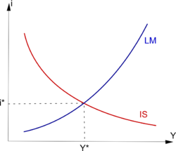
Figure 2 - IS/ LM model

So, we can see that the IS curve is sloping downward. This assumes that the level of consumption/ and investment is negatively correlated with interested rates while being positively correlated with GDP. This is justifiable. For instance, if interest rates increase then the cost of borrowing becomes more expensive, potentially deterring customers and businesses from lending. From the business perspective, increased interest rates will increase the cost of lending for capital expenditure, which in turn may increase the desired rate of return on projects, making some financially unviable. So, another way to consider the IS curve would be as a visual to all the combinations of income (Y) and borrowing ® which equal total supply, shown in the equation below:

Yd(Y, r) = Y

Where the Y on the left-hand side stands for income, r equals the cost of borrowing which could also be seen as the interest rate, and Y on the right-hand side stands for total supply.

By contrast, the LM curve slope upwards which suggests the quantity of money demanded is positively correlated to interest rate. So, another way to image the LM curve would be as a visual to all the combinations of Y and r which equilibrate to the money market, considering the price level (P) and money supply (M), shown in the equation below:

Md(Y,r) =M/P

Examples can be presented into how the IS/LM curve would react to changes in the market. For instance, the graph below shows an example whereby a rise in consumer spending shifts the IS curve to the right-hand side; note that a decline would see the curve move in the opposite direction. For any given interest rate, the aggregate demand function shifts downward, the equilibrium level of aggregate output falls, and the IS curve shifts to the left.

Other factors can also impact on the IS curve; namely investment, exports, government spending and taxation. While there are five main factors which can impact on the IS curve, there are two main factors which may impact on the LM curve. These can be seen as changes in the money supply as well as autonomous changes in money demand; changes which are independent of the current interest rates. So, in the graph below the LM curve is being shifted to the right given an increase in excess money supply:

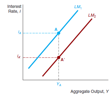
As noted in this example, the idea would be that the excess supply of money would push the interest rates lower; there would be no increase to aggregate output here given that there is no demand for this money; be it for consumer spending, investment etc.

The IS-LM graphs are typically drawn in such a way that the equilibrium interest is positive. However, in recent years the target (short term) interest rates have declined to zero and cannot go further downward (since nominal interest rates for the most part cannot be negative).

In this situation, equilibrium income is Y0, and the interest rate is at 0. An increase in the money supply shifts out the LM curve, but cannot further drive down the interest rate. Since interest rates can’t decline, then investments cannot be encouraged by this channel. However, fiscal policy can increase output which would cause a shift outward of the IS curve. Hence, here, monetary policy becomes ineffective, while fiscal policy has quite an effect.

1.7 Final Comments

To conclude, this chapter has considered income, and expenditure. Essentially, the economy can be seen as a circular flow of cash, mainly between businesses and households. Businesses pay households for working, while the householders then give their money back to the business through spending on goods/ services. However, as mentioned there are several leakages to consider. Taxes are one, however this would be injected back into the economy through government spending as denoted in the consumption functions; namely AD = C + I + G + (X-M). Secondly, we can consider savings from both consumers and businesses. The scale of this would be dependent on the marginal propensity to save; however, in any case it is a withdrawal. Although, what could be mentioned here is that savings do re-enter the economy as banks lend out the money to consumers/ businesses; although there is still some leakage for those hoarding cash at home etc., or through the fact that financial institutions do have to keep a certain level of cash back as capital. Finally, the third leakage mentioned was imports, a major issue for the UK given that the economy remains in a current account deficit, whereby more money is flowing out of the economy than coming in. In this case, economic theory would suggest a change in the value of the national currency would change to bring to the market back into equilibrium. In the case of the UK this should depreciate the national currency, which in turn would make imports more expensive, and exports cheaper for international customers. Theoretically, imports should fall and exports rise until the market balances, creating equilibrium. However, this may not always be the case given a host of other factors to consider given the types of goods needed; i.e. some countries do not have the natural resources to supply their own food/ energy etc., as well as consumer choice and taste.

So, there is the potential that income could continue to leak out of the economy in the long-term. Demand for goods could also come into question here. For instance, we have mentioned that some goods may be elastic in demand, while other inelastic. We can consider this using the UK’s current account deficit as an example. For instance, assume that the UK imports just two goods; oil and chocolate. Oil demand could be considered as inelastic given the need for it in daily life for both consumers and businesses. So, if the UK’s currency depreciated and oil become more expensive, demand wouldn’t fall as much as the % rise in price given that oil is needed for essential duties, be it powering cars or industrial applications. On the other hand, chocolate demand may fall if the price is increased given that the consumer would easily forgo the good, potentially substituting their demand for chocolate for another good.

Practical Example

The following chapter looks to discuss income and expenditure, considering how money flows through the economy, supporting national income. When we talk of the ‘Circular flow of Income Model’ there are two actors in the economy, businesses and households. Essentially, households are employed by businesses to produce goods/ services, then using this income (wages) to spend on the goods/ services produced by these businesses. Income moves in a circular function. However, there are spillages to consider which will impact on the movement of money in the economy. To start, there is government spending, which is supported by tax revenue from consumers and businesses. This is a spillage as the money which is used to pay these taxes cannot be used for spending/ investment. However, the idea here is that the government will inject the money back into the economy. Another spillage could be savings, pulling the money out of this circular flow. Although, with this there is the possibility that banks will inject this money back into the economy by lending it out to consumers/ businesses in the form of borrowing. Even with this though, there is still some leakage which can occur given that (1) borrowers may be a higher rate of interest than savers receive, seen as a profit for the bank which may be based internationally; or (2) the bank may have to keep a specified % of capital buffers, essentially cash held within the central bank which will be seen as non-productive.

Another leakage could be seen as imports, whereby consumers are purchasing goods/ services from abroad, leading to the money leaking from the economy into another. Focusing on the UK for a moment, it could be considered that this is true, with the UK usually running a current account deficits; whereby outflows are higher than inflows.

Moving on, The Keynesian Cross Model could also be considered; shown below,

Figure 3- Keynesian Cross Model

The graph depicts the relationship between aggregate demand and real GDP, denoted as (Y). The curve is drawn upward sloping given the expectation that as (Y) increases, consumers have higher disposable income, which in turn will allow them to demand more goods/ services.

On the Keynesian Cross model, you will notice that there is a 45-degree line drawn in. This is because the goods market always comes into equilibrium, like mentioned above, if planned expenditure (demand) is running ahead of firms’ production, then their existing inventory stocks get depleted and it encourages them to produce more as they know the demand is there to sell their goods. If demand is below firms’ production then they are just accumulating unsold stocks in their inventories, so they scale their production levels down. Eventually we have a situation where planned expenditure (demand) = actual production (output), so demand equals output (or income). Noting this, the 45-degree line is just because we have drawn Z on one axis and Y on the other, we know that in equilibrium Z=Y which will be somewhere on this 45-degree line. The actual point where it comes into equilibrium will be where the planned expenditure line crosses the 45-degree line.

The point of equilibrium comes when aggregate demand, equals aggregate supply, which as we note can also be determined as national output. The model can also be expressed with the equation shown below:

You may recognise this model; it is simple the aggregate demand function with the (C) for consumption replaced by its components. So in this new equation ‘a’ is noted as the autonomous consumption, and so the planned consumption of the consumer. ‘b’ is then seen as the marginal propensity to consume which would then be determined by total income (Y) minus any taxes which need to be paid. Essentially, the total consumption of the consumer will be determined by (1) their planned consumption which would be based on the income expectations, added with (2) the marginal propensity to consumer any further unexpected income.

Another model which can be considered here is the Multiplier Effect, which will consider in this case how money can be multiplied in the economy to create a much larger impact on output. For instance, consider a worker being paid £100 who then spends the £100 in the local economy. The money moves through the economy to local business, who then potentially spend this money on wages/ invested, then creating new income in the economy to be spent once again. Suddenly, the £100 can be multiplied in the economy several times over.

In any case, the expectation would be that equilibrium should be reached. When it comes to determining the equilibrium, this will be dependent on supply/ demand of a good or service. The equilibrium will be reached when the price/ output reach a point whereby the demand from consumers is balanced with the supply from businesses. It could be noted that each are driven by conflicting factors. For instance, if the price is higher, firms would be incentivised to supply more to increase their earrings. However, higher prices would deter demand from consumers; consumers would be more willing to buy if the price is low. So, a compromise must be found which can be referred to as the equilibrium.  This is where output could be maxmised in economy to match demand.

Moving on, the chapter then considers the IS/ LM model, a diagram which considers two curve, being the ‘Investment Savings’ and ‘Liquidity Money’. The three critical exogenous variables in the IS-LM model are liquidity, investment and consumption. Per the theory, liquidity is determined by the size and velocity of the money supply. The levels of investing and consumption are determined by the marginal decisions of individual actors. The IS curve can be considered as a variation of the income-expenditure model which also brings into consideration interest rates and how this impacts on the economy. So, the IS curve assumes that the level of consumption/ and investment is negatively correlated with interested rates while being positively correlated with GDP. This is justifiable. For instance, if interest rates increase then the cost of borrowing becomes more expensive, potentially deterring customers and businesses from lending.

To provide a definition, the income-expenditure model was developed by John Maynard Keynes to explain the fluctuations in spending and the production of goods/ services. Basically, the model states that the production of goods will match the demand which could be sold. Ultimately, this will lead to equilibrium; keeping the economy stable.

Moving on, the LM curve represents the amount of money available. The LM curve slope upwards which suggests the quantity of money demanded is positively correlated to interest rate. This seem logical given that idea that higher interest rates would increase the supply of money onto the market; i.e. image that banks will be willing to supply more money to consumers/ businesses as they can now earn higher interest on these loans.

So, the point at which these two curve meet would be an equilibrium where the supply of money equals the demand.