Fiscal Policy and Current Account Balance: An Empirical Analysis for Thailand

Fiscal Policy and Current Account Balance: An Empirical Analysis for Thailand

Research Proposal

1. Introduction and Motivation

During the pre-2000 period, Thailand has achieved remarkable progress in developing its economy and society. Its annually average Growth Domestic Product (GDP) growth rate was 7.5% during the period from 1960 to 1996, and it has been called the “Fifth Tiger” (Warr,1999). What’s more, Thailand has actively participated in global and regional economic events and organizations. In 1949, Thailand became a member of both the World Bank and the International Monetary Fund (IMF). Also, Thailand is one of the founders of the Association of Southeast Asian Nation (ASEAN), the Asia-Pacific Economic Cooperation forum (APEC) and the Asian Development Bank (ADB), and it got accepted by the World Trade Organization (WTO) in 1995. All of these facts illustrate how important Thailand is towards Southeastern Asia and the whole world.

Despite achieving such extraordinary developing progress, the Thai economy started to face severe challenges since the late 1990s. In 1997, the Asian Financial Crisis took place. The GDP growth rate for Thailand quickly dropped to negative values for the following two years. In addition to that, Thailand had a very low annual average GDP growth rate, 3.05%, for the 2008 – 2015 period because of the Global Financial Crisis in 2008.

To solve such an issue and regain market prosperity, the Thai government began to intensively implement expansionary fiscal policies.  In 1998, right after the Asian Financial Crisis, Thailand started to have a government budget deficit equaled to 2.9% of its GDP. Then, Thailand had an even higher Government budget deficit equaled to 4.7% of its GDP in 2009. Furthermore, as a consequence of its rapidly increasing budget deficit, the Thai government is also experiencing dramatically growing government debt. The government debt was only the same as 15.2% of its GDP in 1996, but the average government debt to GDP ratio became 44.4% from 1996 to 2016.This percentage is not extremely high but raising with extraordinary speed. ¹

In 2017, Thailand announced the 20-year national strategy and claimed to obtain developed country status in 2036.² With only a GDP growth rate 3.9% in 2017 and all the facts we described above, it is very intriguing to study and analyze whether Thailand can truly recover from the wound, the financial crisis had brought to its economy, and accomplish such a target. And with this purpose in our mind, it is especially important to figure out what is the real connection between Thailand’s fiscal position and its current account balance, for the former is the major tool that the Thai government is using to cure and stimulate its economic system, and the latter is a direct measurement of the Thai external balance condition.

We found that Ahmad and Evan’s paper (2007) discussed the same topic in their paper, but their data is from 1976 to 2001, which can not give us informative knowledge about the situation in Thailand for the most recent two decades. Thus, in this paper, we will focus on the fiscal policy and current account balance for the 1993 – 2010 period. With data from this time period, we can capture information about how government spending, especially budget deficit, affects the current balance after both financial crisis (1997,2008). Also, in the paper, I will use trade balance and current account balance interchangeably since they share a similar pattern in Thailand, just like Figure 1 shows.

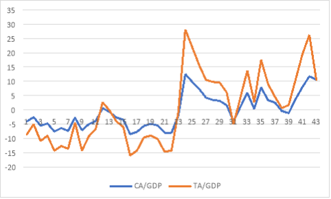
Figure 1: Current Account (CA) and Trade Account (TA) Balance as a percentage of GDP in Thailand (1975 – 2017)

2. Research Purposes

This paper will analyze fiscal policy in Thailand and its impact on Thai current account balance in the 1993 – 2010 period by answering the following question:      

1. Does the effect of the Thai government budget balance on its current account balance follow the twin deficit, the twin divergence, or the Ricardian Equivalence hypothesis?

3. Theory and Related Literature

The real effect between a country’s fiscal policy and its current account balance is very hard to determine. This is because of the complicated impact that fiscal policy will trigger on each component of the current account balance. In concept, the current account balance equals to national saving less investment and plus some non-negligible statistical discrepancies. Then, we can divide national saving into private saving and government saving, which is also known as the government budget balance. The same separation is applied to the national investment, and we can get the following equation:

Current Account = National Saving – National Investment + Statistical Discrepancy

                            = private saving + government budget balance

                             – private Investment – government Investment + Statistical Discrepancy

According to the equation, we can easily detect the positive correlation between the current account balance and the government budget balance. In other words, the current account deficit and budget deficit must also move in the same direction. This phenomenon is called the “twin deficit”. As shown by the standard Mundell-Fleming model, for a small open economy, an increase in budget deficit tends to cause the interest rate to move upward. Then, the higher interest rate will lead to capital inflows and appreciation of the exchange rate. Eventually, the small open economy’s net exports will drop and so will the current account balance since the domestic currency becomes more expensive. In empirical works, adjusted international real business cycle models (e.g., Baxter, 1995; Kollmann, 1998; Erceg, Guerrieri, and Gust, 2005) also confirm such correlation exists between the government budget deficit and current account deficit.

Nevertheless, many economists hold views different from twin deficit. Firstly, empirical findings show that the precise effects of fiscal policy on the current account highly depend on some crucial factors. For instance, according to the intertemporal model (Obstfeld, Rogoff, 1995), if an increase in government expenditure happens, then the trade balance will be worse only when the increase is temporary. And no obvious impact on the trade balance can be detected if the increase in government spending is permanent.

What’s more, Kim and Roubini (2008) report a finding implies that the twin deficit hypothesis does not fit the data in the U.S. They claim that, for the post-Bretton Woods period of flexible exchange rates, their result shows that expansionary fiscal shocks, or the government budget deficit shocks, are actually related to an improvement of the current account balance. And this result is true even if they control the business-cycle and output-shocks, which usually are the reason why such a negative correlation exists. This correlation between the government budget deficit and current account deficit is known as the “twin divergence” phenomenon. Similar to the U.S case, Kim and Lee (2018) also claim that the twin deficit phenomenon only appears in Korea for the pre-2000 sample period. And for the post-2000 period, Korean trade balance drops persistently and significantly in response to the government spending shock.

Lastly, the rest economists believe in the Ricardian Equivalence hypothesis and they assert that “shifts between tax-financed and debt-financed government spending have no effect on macroeconomic aggregates and prices.” (Kimbrough and Gardner, 2019). Ricardian scholars claim that rational public will always anticipate a raise on the tax in the future after a cut on the tax at present. Therefore, people tend to consume less and save more to balance their disposable income for the whole time period. Ultimately, the private sector wealth and the government spending will not be changed, which implies that the trade balance is not affected either.

4. Methodology

We will determine our model and get the empirical result by following the beneath procedure:

1) First, we need to implement integrational tests on each of our variables. These variables can be either unit root or trend stationary, and we can test them by exploiting the Dickey-Fuller test (1981).

2) After knowing stationary properties of these variables, we need to determine the optimal lag length for each series of our variable. This purpose will be achieved by trying different lag lengths when implementing the Dickey-Fuller test and select the one that gives us the lowest value of Akaike Information Criteria (AIC) and Bayesian Information Criteria (BIC).

3) Then we need to test for cointegration based on the Johansen and Juselius (1990) method. It is important to make the degree-of-freedom adjustment for this test because this test excessively tends to falsely reject the null hypothesis that no cointegration exists. And we will use the Reinsel and Ahn (1992) correction factor (T- nk)/T, where T is the total number of observations, n is the number of variables in the system and k is the lag length. In the end, we will multiply this factor with the test statistics to get our adjusted statistics.

4) Next, we will do the granger-causality test based on previous results. If cointegration does exist, we will have to employ the vector error correction model (VECM) in the aim of capturing the real long run connection between budget deficit and current account deficit in Thailand. Otherwise, we can just estimate the standard log difference vector autoregressive (VAR) model.

5) Finally, after the above four steps, we will estimate our model and get the orthogonalized impulse-response functions (OIRF) based on Cholesky decomposition. Then we can determine the true relationship between the Thai fiscal policy and the current account balance based on these OIRFs. One thing we need to pay attention here is that the OIRFs are usually sensitive to the order of variables, but we will show how we can solve this issue in the model section.

5. Model (1p – 2p)

If cointegration does not exist, then we will employ the following VAR model:

${\mathit{x}}_{\mathit{t}}= \sum _{j=1}^p{\mathbf{\Phi }}_{\mathit{j}}{\mathit{x}}_{\mathit{t}\mathit{–}\mathit{j}}+ {\mathit{C\epsilon }}_t$

,                                               (1)

where

${\mathit{x}}_{\mathit{t}}=[ \begin{array}{cc}{g}_t& {\mathit{z}\mathit{‘}}_{\mathit{t}}]‘\end{array}$

                                                       (2)

and $g_t$

infers to a measurement of government spending such as the government budget balance. ${\mathit{z}}_{\mathit{t}}$

is as following:

${\mathit{z}}_{\mathit{t}}\mathbf{=}\mathbf{[}\begin{array}{ccc}{y}_t& {\mathit{cab}}_t& {\mathit{nir}}_t\end{array}\mathit{ }\begin{array}{cc}{\mathit{inf}}_t& {\mathit{ner}}_t]‘,\end{array}$

                                     (3)

where $y_t$

is a measure of private spending such as household consumption or private investment, ${\mathit{cab}}_t$

is the current account balance as a share of total GDP, ${\mathit{nir}}_t$

is the nominal interest rate, ${\mathit{inf}}_t$

is the inflation rate, ${\mathit{ner}}_t$

is the nominal exchange rate denominated in US dollar, C is a lower-triangular matrix and ${\epsilon }_t$

is a vector of mutually orthonormal structural shocks. Also, ${\mathit{x}}_{\mathit{t}}$

is demeaned and detrended before estimation.

One thing we need to notice is we solve the issue about OIRF by assigning  $g_t$

as the first term in ${\mathit{x}}_{\mathit{t}}$

, and assumes that government spending variable is not affected by variables in ${\mathit{z}}_{\mathit{t}}$

within one quarter. This assumption is widely used in fiscal policy papers, and it is reasonable because implementing fiscal policies normally needs congressional approval. More detailed and theoretical explanations are in Kim, Kim, and Stern (2015).

Then, if cointegration does exist for two or more series of data in our case, we will employ the VECM. The reason is that series that are cointegrated tend to move together in the long run. Thus, a first-difference VAR model can provide us with the covariance-stationary condition, yet it can not capture the long-run patterns we want.

A VECM is just a restricted form of normal VAR model plus a lagged error-correction term:

${\mathit{∆}\mathit{x}}_{\mathit{t}}= \mathrm{\Psi }{\mathit{x}}_{\mathit{t}\mathit{–}\mathit{1}}+\sum _{i=1}^{p–1}{\mathbf{\Theta }}_{\mathit{i}}{\mathit{∆}\mathit{x}}_{\mathit{t}\mathit{–}\mathit{i}}+ {\mathit{C\epsilon }}_t$

,                                    (4)

where

  ${\mathit{∆}\mathit{x}}_{\mathit{t}\mathit{–}\mathit{i}}= {\mathit{x}}_{\mathit{t}\mathit{–}\mathit{i}}\mathit{–}\mathit{ }{\mathit{x}}_{\mathit{t}\mathit{–}\mathit{i}\mathit{–}\mathit{1}}\mathit{ }$

(5)

$\mathrm{\Psi }=\mathrm{ }\mathit{ }\sum _{j=1}^p{\mathbf{\Phi }}_{\mathit{j}}\mathit{–}\mathit{Identity\; matrix}$

                                 (6)

${\mathbf{\Theta }}_{\mathit{i}}\mathit{=}\mathit{ }\mathit{–}\sum _{j=i+1}^p{\mathbf{\Phi }}_{\mathit{j}}$

                                                            (7)

All the variables are the same as we used in VAR model (1), and we will also transform those variables that are non-stationary into first differences form.

6. Data

We will use quarterly data of Thailand from the 1993Q1 – 2010Q4 period in our analysis. All the data, except the government budget, are obtained from International Financial Statistics websites, published by the IMF. And data about the Thai government budget is obtained from the Bank of Thailand.  Again, ${\mathit{cab}}_t$

is the current account balance as a share of total GDP. And all the spending variables, the government budget balance ( $g_t)$

, the private consumption ( $y_t)$

will be divided by GDP deflator and then log transformed. We will use the discount rate representing the short-term nominal interest rate ${\mathit{nir}}_t$

, and ${\mathit{ner}}_t$

is the nominal exchange rate denominated in US dollar. Lastly, ${\mathit{inf}}_t$

is Consumer Price Index (CPI) inflation rate that we found. All variables that are in unit of currency are expressed in Thai baht.

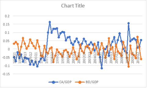
Figure 2: Current Account (CA) balance and Budget Balance (BB) as a percentage of GDP in Thailand (1993Q1 – 2010Q4)

As Figure 2 shows, current account balance and budget balance for the 1993Q1 – 2010Q4 period tend to move in the opposite direction during the whole time. Therefore, it seems plausible to conclude that Thailand follows the twin divergent phenomenon. We will do formal confirmation in the paper later.

7. Paper Organization

The paper will follow the structure:

1)     Introduction

2)     Theory overview and Literature Review

3)     Methodology and data. In this part, we will discuss the model, and we will also describe the data

4)     Empirical results and robustness check analysis

5)     Conclusion and further discussions

References:

• Ahmad Zubaidi Baharumshah, and Evan Lau, 2007. “Dynamics of fiscal and current account deficits in Thailand: an empirical investigation”, Journal of Economic Studies, Vol. 34 Issue: 6, pp.454-475
• Baxter, M., 1995. “International trade and business cycles. In: Grossmann, G.M., Rogoff, K”. (Eds.), Handbook of International Economics, vol. 3. Amsterdam, North-Holland, pp. 1801–1864.
• Dickey, D.A and Fuller, W.A., 1981. “Likelihood Ratio Statistics for Autoregressive Time Series with a Unit Root”, Econometrica,Vol. 49.
• Erceg, C.J., Guerrieri, L., Gust, C., 2005. “Expansionary Fiscal Shocks and the Trade Deficit”. International Finance Division Discussion Paper No.825, Federal Reserve Board.
• Johansen, S. and Juselius, K., 1990. “Maximum likelihood estimation and inference on cointegration with application to the demand for money”, Oxford Bulletin of Economics and Statistics, Vol. 52, pp. 169-210.
• Kim, H., J. Kim, and M. Stern, 2015. “On the Robustness of Recursively Identi.ed VAR Models”. Working Paper.
• Kimbrough, Kent P. and Gardner, Grant W., Notes on International Economics, Chap.13
• Kim, H, and Lee,D., 2018. “The effects of government spending shocks on the trade account balance in Korea”, International Review of Economics and finance, 53, 57 – 70
• Kim, S., and Roubini, N., 2008. “Twin deficit or twin divergence? Fiscal policy, current account, and real exchange rate in the U.S”, Journal of International Economics, 97, 436-447
• Kollmann, R., 1998. “U.S. trade balance dynamics: the role of fiscal policy and productivity shocks and of financial market linkages”. Journal of International Money and Finance 17, 637–669.
• Obstfeld, Maurice and Rogoff, Kenneth., 1995 “The Intertemporal Approach to the Current Account.”  In G.M. Grossman and K. Rogoff, Handbook of International Economics, Amsterdam: North-Holland, pp. 1731-1799.
• Reinsel, G.C. and Ahn, S.K.,1992. “Vector autoregressive models with unit roots and reduced rank structure: estimation, likelihood ratio test and forecasting”, Journal of Time Series Analysis, Vol. 13, pp. 353-75.
• Warr, P.G. (1999), “What happen to Thailand?”, Working Paper in Trade and Development No. 3, The Australian National University, Canberra.