Effects of Free Trade Agreements on Trade and Growth in US
| ✅ Paper Type: Free Essay | ✅ Subject: Economics |
| ✅ Wordcount: 1989 words | ✅ Published: 29 Aug 2017 |
|
The Effects of Free Trade Agreements on Trade and Growth in American Countries: Evidence from the Gravity Model Approach |
Trade as a driver of growth and development is a concept that has been addressed from different perspectives or approaches for scholars and policy-makers. However, an integrative path was sealed with the creation of the World Trade Organization as the main tool to promote a more accessible and clear way to commerce between nations and was further strengthened by bilateral and multilateral FTAs, which continue developing and growing.
In the current political scenario, the discussion between supporters of globalisation and detractors provides a compelling framework to study the real effects that Free Trade Agreements cause on the economic performance. While the first group affirms that FTAs enhances the markets and therefore, the economic growth and employment, the second group argues that the global market is damaging the small domestic economies.
The present paper covers the increasing effects on trade that are expected by countries that engage in Free Trade Agreements, including bilateral or multilateral ones within American countries, in the context of the three central multilateral trade agreements in the continent (NAFTA, MERCOSUR, and The Pacific Alliance) and other relevant bilateral agreements. The main question to be addressed is whether the positive effects predicted by economic theory on trade when countries eliminate fares and other barriers to trade as part of an agreement effectively happen in the current context of the Americas. The hypothesis is that the implementation of Free Trade Agreements has a positive and significant impact on the trade flows between the American countries. Section 2 includes the theoretical framework behind the relation between trade and FTAs, Section 3 presents the model specification, Section 4 shows the estimation of the model and the econometric tests, the limitations of the theoretical framework and the model specification are discussed in Section 5, and Section 6 concludes.
The Gravity Model has its origins on Location Theory, as it was the main model to include the effects of distance on traded quantities. Isard and Peck (1954) acknowledged the importance of considering distance as a variable in trade analysis establishing the ground from which others such as Tinbergen (1962) and Pöyhönen (1963) would build the Gravity theory to explain trade flows between countries, conducting the first econometric studies based on the gravity equation.
The Gravity Model has proven to be extremely successful in ordering the observed variations in economic transactions and movement of factors. It is also distinguished for its representation of economic interaction in a multi-country world, where the distribution of goods and factors is driven by gravity forces that are conditional to the size of economic activities at each location (Anderson, 2010). In this way, trade between countries is positively related to countries sizes and negatively related to distance. Moreover, as a widely used analytical framework, the model can incorporate adjusting variables such as FTA to indicate the existence of Free Trade Agreements between the objective countries (Yang and Martinez-Zarzozo, 2014).
Tinbergen (1962) suggests an economically insignificant “average treatment effects” of FTAs. However, numerous studies, such as Frankel (1997) on MERCOSUR, find a significant positive effect in line with the expected results. These contradictory outcomes emphasise the fragility of the estimation of FTAs treatment effects and are a clear signal that robustness should be tested.
One of the central issues to be explored is the exogeneity of FTAs, since the presence of them, if endogenous, can provide seriously biased results. Baier and Bergstrand (2007) provide several important conclusions to be taken into consideration. They observe that using the standard cross-section gravity equation provides a downwards-biased result. Secondly, attributed to this bias, traditional FTAs effects are underestimated by around 75%-85%. Lastly, the authors demonstrate that the best estimates of the effect of FTAs on bilateral trade are achieved from a theoretically framed gravity equation using panel data with bilateral, country and time fixed effects or differenced panel data with country and time effects.
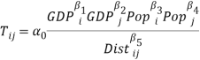
As it is suggested by extensive literature, trade flows are better explained by the Gravity Model, which propose the Newton’s Gravity concept to explain bilateral trade as an attraction force, influenced positively by the size of the economies involved in trading and negatively with the costs of transaction (Tinbergen, 1962 and Pöyhönen, 1963). As proxy variables of the size of the economy, the model uses GDP and population of both countries; and Distance between the countries as a proxy for transaction costs. Following the Newton’s Gravity Equation, the model estimates:
Where  is the trade flows between a specific country pair, in other words, is the sum of exports from country
  to country
  plus exports from country to country .
  is the gross domestic product in country ,
  is the population of country ,
  is the GDP in country ,
  is the population of country , and
  is the distance between the capital cities (as major economic centres) of countries and . To avoid spurious effects due to inflation and currency exchange rates, the variables , and are measured in 2010 constant US dollars.
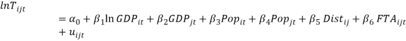
Moreover, recent literature has implemented an augmented version of the gravity model to evaluate other variables of interest related to trade flows. In this way, besides to include more time-sections to the analysis, a dummy for implemented FTAs is added to the explanatory variables, taking a value of 1 if there exist a fully in force agreement and 0 otherwise. For the purpose of this paper, an FTA is considered if it establishes 100% free trade, because many cooperation agreements in the Americas consider only certain sectors for free trade, and these are not the focus of this research. Including the dummy variable, transforming the gravity model using Logarithmic function, to accomplish the linearity-in-parameters assumption, and including the time sections, the model to estimate is:
However, it is strongly likely that this model has problems of endogeneity and thus, the estimators  are biased due to sampling selection and omitted variable bias, how it is suggested by the literature. However, the logic behind this biasedness is different to the literature review. For Baier and Bergstrand (2007), the parameter of interest
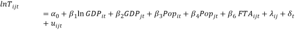
  would have a negative bias because countries will be more interested in implementing an FTA when the benefits of it are greater. Therefore, the authors conclude that a possible omitted variable would be Tariff Barriers. In this scenario, Tariff Barriers are negatively correlated with trade and positively with FTA, generating a negative bias. This is not the case for America. On the contrary, progressive lower barriers and an improving in the diplomatic relationships have finally pushed the creation of Free Trade areas and agreements. That is why, in this case, we suggest that the bias for the sample would be positive, since the possible omitted variables would be lower barriers and good diplomatic relationships, affecting the FTAs and the trade itself positively. To solve this problem, the literature suggests the use of Fixed Effects Panel Data strategy because this model can control for country-specific and invariant-in-time unobservable variables. Therefore, the model to estimate is:

Where  will be the identifier for the 29 different country-pair units. Since the Fixed Effects model reacts only to variant-in-time variables, the variable Distance is dropped from the model. This estimation allows controlling by characteristics related to the specific country-pair like diplomatic relationships, trade openness, institutions, and so on. However, there could be variables related to unobserved characteristics in time like trade trends and generalised willingness to trade and sign FTAs. For this reason, it is recommended to use time fixed effects to avoid endogeneity, through the next model:
Where  will be the identifier for the 13 different time sections.
Since the scope of this paper is to evaluate the effect of the FTAs on American countries, the three biggest trade agreements in the continent (NAFTA, MERCOSUR, The Pacific Alliance) were taken as a research target, and their members were chosen as the population. The countries included by Trade Agreement are presented in Table 1:
Table 1. Multilateral Trade Agreements in America
|
Agreement |
Country |
Start Date |
|
North American Free Trade Agreement (NAFTA) |
Canada |
01/01/94 |
|
Mexico |
01/01/94 |
|
|
United States |
01/01/94 |
|
|
Southern Common Market (MERCOSUR) |
Argentina |
15/08/91 |
|
Bolivia |
28/02/97 |
|
|
Brazil |
15/08/91 |
|
|
Paraguay |
15/08/91 |
|
|
Uruguay |
15/08/91 |
|
|
MERCOSUR – Chile |
Chile |
01/10/96 |
|
The Pacific Alliance |
Chile |
01/02/12 |
|
Colombia |
01/02/12 |
|
|
Mexico |
01/02/12 |
|
|
Peru |
01/02/12 |
Source: Organization of American States (2016)
However, if those countries were incorporated without taking into account other Free Trade Agreements between them or third countries, problems of sample selection bias would be created. For this reason, in addition to the mentioned free trade areas, bilateral FTA are considered, according to Table 2:
Table 2. Bilateral Trade Agreements in the sample
|
FTA |
Start Date |
|
|
Bolivia |
Mexico |
07/06/10 |
|
Canada |
Chile |
05/12/96 |
|
Canada |
Colombia |
21/11/08 |
|
Canada |
Peru |
29/05/08 |
|
Chile |
Mexico |
01/08/99 |
|
Chile |
Panama |
07/03/08 |
|
Chile |
Peru |
01/03/09 |
|
Mexico |
Chile |
01/08/99 |
|
Mexico |
Uruguay |
15/07/04 |
|
Panama |
Canada |
01/04/13 |
|
Panama |
Peru |
01/05/12 |
|
United States |
Chile |
01/01/04 |
|
United States |
Colombia |
15/05/12 |
|
United States |
Panama |
31/10/12 |
|
United States |
Peru |
01/02/09 |
Source: Organization of American States (2016)
As the model considers only one dummy variable, if a country-pair has two agreements in force (bilateral and trade area), it is considered the oldest one. Besides, it is important to point out that Venezuela (suspended member of MERCOSUR) was dropped from the list due to the lack of reliable information about trade flows. The information about bilateral trade flows was obtained from The World Bank’s World Integrated Trade Solution, and the other variables were constructed using information from the World Development Indicators. The database used to estimate the model has 29 country-pairs (cross-sectional units) and 13 time-sections since 1990 to 2014. The used database of bilateral trade drops 1996, leaving the database with one time-section less. Since it is one time-section of fourteen and according to our investigation, the missing information is not related to an event influencing trade flows and the time section is dropped for the entire observations, we have a low risk of biased estimators.
Table 3 contains the descriptive statistics showed by the Statistical Software STATA® for the variables in levels:
Table 3. Descriptive statistics of relevant variables (in levels)
|
| |
Mean |
Std. Dev. |
Min |
Max |
| |
Observations |
||
|
ID |
overall |
| |
25.45435 |
19.18174 |
1 |
74 |
| |
N = 460 |
|
between |
| |
19.36072 |
1 |
74 |
| |
n = 29 |
||
|
within |
| |
0 |
25.45435 |
25.45435 |
| |
T-bar = 15.8621 |
||
|
| |
| |
|||||||
|
Exports |
overall |
| |
4.55E+10 |
1.22E+11 |
1.45E+08 |
6.13E+11 |
| |
N = 460 |
|
between |
| |
1.01E+11 |
4.22E+08 |
4.75E+11 |
| |
n = 29 |
||
|
within |
| |
3.63E+10 |
-1.67E+11 |
2.48E+11 |
| |
T-bar = 15.8621 |
||
|
| |
| |
|||||||
|
GDP_Exp |
overall |
| |
1.02E+12 |
2.25E+12 |
9.96E+09 |
1.62E+13 |
| |
N = 460 |
|
between |
| |
2.40E+12 |
1.37E+10 |
1.30E+13 |
| |
n = 29 |
||
|
within |
| |
3.60E+11 |
-1.94E+12 |
4.21E+12 |
| |
T-bar = 15.8621 |
||
|
| |
| |
|||||||
|
Pop~Exp |
overall |
| |
6.71E+07 |
7.28E+07 |
2738125 |
3.19E+08 |
| |
N = 460 |
|
between |
| |
7.16E+07 |
3324953 |
2.86E+08 |
| |
n = 29 |
||
|
within |
| |
8255115 |
3.64E+07 |
9.97E+07 |
| |
T-bar = 15.8621 |
||
|
| |
| |
|||||||
|
GDP_Imp |
overall |
| |
6.78E+12 |
6.55E+12 |
9.96E+09 |
1.62E+13 |
| |
N = 460 |
|
between |
| |
6.28E+12 |
1.61E+10 |
1.38E+13 |
| |
n = 29 |
||
|
within |
| |
1.50E+12 |
2.71E+12 |
1.00E+13 |
| |
T-bar = 15.8621 |
||
|
| |
| |
|||||||
|
Pop~Imp |
overall |
| |
1.68E+08 |
1.31E+08 |
3201604 |
3.19E+08 |
| |
N = 460 |
|
between |
| |
1.31E+08 |
3310046 |
2.95E+08 |
| |
n = 29 |
||
|
within |
| |
1.42E+07 |
1.31E+08 |
2.00E+08 |
| |
T-bar = 15.8621 |
||
|
| |
| |
|||||||
|
FTA |
overall |
| |
0.5043478 |
0.5005254 |
0 |
1 |
| |
N = 460 |
|
between |
| |
0.4360526 |
0 |
1 |
| |
n = 29 |
||
|
within |
| |
0.2546286 |
-0.453985 |
1.393237 |
| |
T-bar = 15.8621 |
||
|
| |
| |
|||||||
|
Distance |
overall |
| |
3690.712 |
2529.406 |
213.02 |
8483.39 |
| |
N = 460 |
|
between |
| |
2533.405 |
213.02 |
8483.39 |
| |
n = 29 |
||
|
within |
| |
1.55E-12 |
3690.712 |
3690.712 |
| |
T-bar = 15.8621 |
However, since the estimations are calculated using a logarithmic transformation of the continuous variables, the descriptive statistics of the variables in natural logarithm are presented in Table 4:
Table 4. Descriptive statistics of relevant variables (in logarithm)
|
Variable |
| |
Mean |
Std. Dev. |
Min |
Max |
| |
Observations |
|
|
FTA |
overall |
| |
0.5043478 |
0.5005254 |
0 |
1 |
| |
N = 460 |
|
between |
| |
0.4360526 |
0 |
1 |
| |
n = 29 |
||
|
within |
| |
0.2546286 |
-0.4539855 |
1.393237 |
| |
T-bar = 15.8621 |
||
|
| |
| |
|||||||
|
lexports |
overall |
| |
2.25E+01 |
1.84E+00 |
1.88E+01 |
27.14178 |
| |
N = 460 |
|
between |
| |
1.64E+00 |
1.98E+01 |
26.85607 |
| |
n = 29 |
||
|
within |
| |
5.17E-01 |
2.10E+01 |
23.84729 |
| |
T-bar = 15.8621 |
||
|
| |
| |
|||||||
|
lGDP_ex |
overall |
| |
2.65E+01 |
1.66E+00 |
2.30E+01 |
30.41464 |
| |
N = 460 |
|
between |
| |
1.69E+00 |
2.33E+01 |
30.18564 |
| |
n = 29 |
||
|
within |
| |
2.28E-01 |
2.58E+01 |
27.04886 |
| |
T-bar = 15.8621 |
||
|
| |
| |
|||||||
|
lGDP_im |
overall |
| |
2.77E+01 |
2.795514 |
2.30E+01 |
30.41464 |
| |
N = 460 |
|
between |
| |
2.719438 |
2.35E+01 |
30.25019 |
| |
n = 29 |
||
|
within |
| |
1.94E-01 |
2.70E+01 |
28.17505 |
| |
T-bar = 15.8621 |
||
|
| |
| |
|||||||
|
lPop_ex |
overall |
| |
1.75E+01 |
1.11E+00 |
1.48E+01 |
19.58041 |
| |
N = 460 |
|
between |
| |
1.12E+00 |
1.50E+01 |
19.47142 |
| |
n = 29 |
||
|
within |
| |
8.70E-02 |
1.72E+01 |
17.64414 |
| |
T-bar = 15.8621 |
||
|
| |
| |
|||||||
|
lPop_im |
overall |
| |
1.80E+01 |
1.821994 |
1.50E+01 |
19.58041 |
| |
N = 460 |
|
between |
| |
1.826536 |
1.50E+01 |
19.50204 |
| |
n = 29 |
||
|
within |
| |
8.05E-02 |
1.78E+01 |
18.19405 |
| |
T-bar = 15.8621 |
||
|
| |
| |
|||||||
|
ldista~e |
overall |
| |
7.89E+00 |
9.17E-01 |
5.36E+00 |
9.045865 |
| |
N = 460 |
|
between |
| |
9.10E-01 |
5.36E+00 |
9.045865 |
| |
n = 29 |
||
|
within |
| |
0.00E+00 |
7.89E+00 |
7.891049 |
| |
T-bar = 15.8621 |
Although using pooled OLS with the database will generate problems of endogeneity discussed further below, OLS estimation is made to have the first approach to the gravity model. Table 5 shows the obtained results:
Table 5. Gravity Model estimated by OLS
|
lexports |
| |
Coef. |
Std. Err. |
t |
P>|t| |
[95% Conf. |
Interval] |
|
lGDP_exp |
| |
0.6340649 |
0.0394767 |
16.06 |
0 |
0.5564848 |
0.7116451 |
|
lGDP_imp |
| |
0.4512511 |
0.0464715 |
9.71 |
0 |
0.3599247 |
0.5425775 |
|
lPop_exp |
| |
0.2196251 |
0.0606458 |
3.62 |
0 |
0.1004432 |
0.3388071 |
|
lPop_imp |
| |
0.5049373 |
0.0726212 |
6.95 |
0 |
0.362221 |
0.6476536 |
|
FTA |
| |
0.5136195 |
0.0689928 |
7.44 |
0 |
0.3780338 |
0.6492052 |
|
ldistance |
| |
-0.9256142 |
0.0407673 |
-22.7 |
0 |
-1.005731 |
-0.8454978 |
|
_cons |
| |
-12.68833 |
0.7146799 |
-17.75 |
0 |
-14.09283 |
-11.28383 |
With a  , the model behaves according to the literature and all variables are statistically significant using any level of significance. The variables measuring the mass of the economies are positive and distance is negative. Additionally, the variable of interest FTA is positive and statistically relevant, showing tha
Cite This Work
To export a reference to this article please select a referencing stye below:
Related Services
View all


DMCA / Removal Request
If you are the original writer of this essay and no longer wish to have your work published on UKEssays.com then please click the following link to email our support team:
Request essay removal