Theories of Growth Convergence
| ✅ Paper Type: Free Essay | ✅ Subject: Economics |
| ✅ Wordcount: 1241 words | ✅ Published: 04 Oct 2017 |
The purpose of this chapter is to introduce the neo classical theoretical framework which is the basic foundation for the convergence theorem of economic growth. Further, we will see the other major theorems studying growth convergence.
The Neo-Classical Growth Model
“The art of successful theorizing is to make the inevitable simplifying assumptions in such a way that the final results are not very sensitive…and it is important that crucial assumptions are reasonably realistic” (Solow,1956)
The Solow-Swan model, as it is alternatively called is explained in the following 10 equations as done in Barro, Sala-i-Martin(1999)
We start by assuming a simplified, Robinson Crusoe type economy where producer and consumer are the same person who owns the inputs as well as the technology to transform inputs to output. The inputs are broadly classified into physical capital, K(t), and labour, L(t). Let`s also assume technology has no or little change over time.
The production function, thus derived, will be of the following form
Y(t) = F[K(t), L(t)],1
where Y(t) is output at time period t. We further assume a one-sector production model in which output Y(t) is a homogenous good which can either be used for consumption ,C(t), or for Investment I(t) to create new units of Physical Capital K(t). The Capital depreciates at the constant rate δ > 0 We also assume that the economy is closed which implies the output equals income and saving equals investment in all periods, t. Further, we assume a constant, positive savings rate s(). Hence, the net increase in physical capital at a point in time equals gross investment less depreciation
Ḱ = I – δ K = s · F(K, L) – δ K,2
where Ḱ is net increase in capital and 0 ≤ s ≤ 1. Equation 2 determines the dynamics of physical capital K for a given level of labour force L. The labour force L(t) varies in accordance with the population growth, worker participation rates and time worked by an average worker. For the simplicity of the model, we assume that population grows at a constant, exogenous rate, Ĺ/L = n ≥ 0 and that everyone works at same intensity. If the number of people is normalized at time 0 to 1 and the work intensity per person is normalized to 1, then the population and labour force at time t equal to
L(t) = ent3
If L(t) is given from equation 3 and technological progress is absent, then equation 2 determines the time paths of capital, K, and output,Y. Hence the production function becomes
Y = F(K,L)4
A production function is neo-classical if it satisfies the following three properties.
- For all K > 0 and L > 0, the production function F(·) exhibits diminishing marginal products with respect to each input ;


- F(·) exhibits constant returns to scale ;
 for all
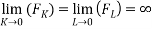
- The Inada conditions are fulfilled ;

The condition 2 implies that the production function can be written in the intensive form as
 ,6
,6
where  and
and 
using the condition  and differentiating with respect to K, for fixed L and then with respect to L, for fixed K, we can rewrite the marginal products of the factor inputs as
 ,7
,7
and 
Satisfaction of Inada conditions imply that
 and
and 
Now we analyse the dynamic behaviour of the economy described by the neo-classical production function.
We recall equation 2. if we divide both sides of the equations by L ;
 8
8
The right side of the above equation has variables written as a function of  while the left side is not. Hence we rewrite Ḱ/L as a function of by using the condition
 ,9
,9
where n= Ĺ/L
if we substitute this result to the expression 9, and rearrange terms to get
 10
10
This nonlinear equation is the fundamental differential equation of Solow-Swan growth model and depends only on .  in the right hand side implies the capital labour ratio,
 ,over time. The term
  is the effective depreciation rate of .
Given a constant saving/investment rate, a decline in capital labour ratio will happen either because of a growth in labour force (denominator value increases) implied by  or because of a fall in capital stock (numerator value decreases) owing to depreciation, denoted by
  .
.
Equation 10 is depicted in the diagram given below. The upper curve, , is the production function in per capita terms. The curve starts from origin since each input is essential for production (Inada Conditions). It gets flatter as rises due to the diminishing marginal returns to capital. The lower curve,
 , represents savings/investment in per capita terms. It starts from origin because
 , it has a positive slope since the marginal productivity of capital is positive (
 > 0) and it becomes flatter because of the operation of diminishing marginal returns to capital (
 < 0).
< 0).
Moreover, the satisfaction of Inada conditions makes  curve vertical when
  .
.
The final term in the equation,  will form a straight line with positive slope due to the assumed constancy of labour force growth and depreciation of physical capital.

The per capital consumption at any point equals the vertical gap between curve and curve at that point. The Per capita investment equals the height of . The vertical distance between curve and line shows the change in the capital labour ratio, . The point where curve and line intersects is called the steady state. In the steady state ( at a positive ), all the important variables in the solow-swan growth equation grows at constant rates.
It is the point corresponding to  At this point,

In the above diagram this point is denoted by k*. Since is constant at k*, the per capita output y as well as the per capita consumption c does not grow as well. Since per capita values of K,Y and C does not grow at steady state, the growth of these variables are entirely dependent on the population growth rate n.
A technological progress, ceteris paribus, will shift the production function  upwards and a proportionate shift in will follow, leading to a higher steady state level of k*. An increase in
  will lead to an upward shift in curve, and with a given production function, this will lead to a higher k*. similarly, an increase in population growth rate or capital depreciation rate will lead to a lower steady state capital labour ratio, k* . However, none of these will lead to a change in per capita growth rates of Y,C or K all of which are equal to Zero. For this reason, the current model does not explain the determinants of the long run per capita growth. Since, according to this model the long run growth rate is entirely determined by exogenous factors, the neoclassical model is also called an exogenous growth model.
Growth Convergence in Solo-Swan Model
In order to understand the idea of convergence, let`s go back to the fundamental growth equation of the Solow-Swan model.
10
Dividing both sides of the equation by k ;
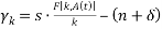
 11
11
 is the growth rate of .
Now,

 is equal to the marginal product of labour which is positive. Hence, the derivative
  will be negative and if plotted in a diagram, will form a downward sloping curve. The second term in the right side of equation will be a positive constant (since we assume and
 to be positive constants)
Equation 11 is depicted below diagram

As is clear from the diagram, every economy in the long run will converge towards the steady state growth rate k*. The farer a country is from this point, the faster the growth rate (positive or negative) and speedier the convergence process will be. If k >k* the growth rate of k will be positive and if k
A noteworthy point here is that the capital-labour substitution process will be faster in poorer countries. This implicitly means that poorer countries have a more labour intensive production process than their richer counterparts. And as the economy grows, the growth rate of capital-labour substitution process falls and in steady state this growth rate is equal to zero. The source of this result is the neo classical assumption of diminishing marginal returns to capital. When k is relatively low, the average product of capital, , and hence the investment per unit of capital,
 , is relatively high. Since the effective depreciation of capital is assumed to be constant, the growth rate of k will also be high. As more are more capital is employed in the production process, the marginal product of capital and consequently the average product will fall, leading to a deceleration in the growth rate of k.
The behaviour of output
In order to study the behaviour output along the convergence process we first define the growth rate of per capita output;
 12
12
The expression in brackets is called the capital share or the share of rental income on capital in total income. The above equation shows that the relation between  and on the basis of the behaviour of capital share.
Now we substitute from Equation 11 for  and we will get
 15
15
Where, 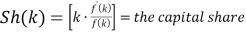
Differentiating equation 15 with respect to and combining terms, we get

Since the capital share is always a positive fraction of the total output, [  ], the last term in the right side of the equation is negative. If
  , then the first term on the right-hand side is non positive and hence
  .
.
Thus,  necessarily falls as rises (and therefore as
  rises) in the region in which , ie., k ≤ k*. this simply means that the growth rate of per capita income falls (though the PCI still rises) as the economy become more capital intensive. This way the growth convergence is proved.
Absolute and Conditional Convergence
The hypothesis that poor economies tend to grow faster per capita than rich ones-without conditioning on any other characteristics of the economies-is referred to as absolute convergence (Barro, Sala-i-Martin, 1999)
The hypothesis that an economy will grow faster the further away it is from its own steady state is referred as the Conditional Convergence. This implies that if a rich economy is further from its steady state than a poor economy from its own steady state is, then, the rich economy would be growing faster than the poor economy. This concept is depicted in the following diagram.
In the diagram below, we consider two economies with different initial stocks of capital per person,  as well as initial saving rates. Here, the absolute convergence hypothesis would predict the poor economy to grow faster than the rich. In the diagram, this would mean a larger distance between
  curve and
  line for the poor country. But this is not true. Here, the rich country would register a higher growth rate in per capita output. This happens because the rich economy has a higher saving rate, and it is possible that
 is further away from its steady state level,
 , than
  from its steady state,
 , is.
, is.

The neoclassical theory of growth does predict that each economy converges to its own steady state and the speed of convergence relates inversely to the distance from the steady state. In other words, the model predicts conditional convergence in the sense that a lower starting value of real per capita income tends to generate a higher per capita growth rate, once we control for the determinants of the steady state.
Technical Progress and convergence
As of now we have assumed that the technology has been constant over time. But this is not true. In fact technology is the most dynamic source of economic progress in an economy. Hence, assuming it to be constant will be an over simplification of the reality. So, we are endogenizing the technology into the model.
There are three methods of doing this. We have to decide whether the technology should be Hicks Neutral, Harrod Neutral or Solow Neutral.
Barro, Sala-i-Martin finds out that only the harrod neutral technical progress, which is labour augmenting, will be consistent with the existence of a steady state, assuming that the technical progress happens in constant rates.
This means the production function takes the form
 ,
,
Where A(t) ≥ 0 is the index of technology. Let`s assume that technology grows at a constant rate, x. The condition for the change in capital stock is

Dividing both sides by L to get
 16
16
Dividing both sides by k
 17
17
the growth rate k depends on the difference between the average product of capital and the effective depreciation rate. The average product of capital, in turn, depends on the constant technological progress at the rate, x. One implication of the above equation is that, since the saving rate,s, population growth rate,n, and rate of depreciation of capital, are constant, and the constant returns to scale assumption has to be maintained, the average product will remain constant only if the capital labour ratio grows at the same pace of the growth rate of technology, i.e., x.
The behaviour of Output
In order to understand the behaviour of output once endogenous technology is incorporated, we first rewrite the production function in per capita terms
 18
18
In the above expression, since both k and A(t) grows at the rate, x, per capita output, y, also grows at the same rate. This means that Consumption [  ] grows at the same rate too. Moreover, since k and A(t) grows at the same rate in steady state, Let

 is called the effective amount of labour.
  is, thus, the quantity of capital per unit of effective labour. Similarly, the quantity of output per unit of effective labour is
 19
19
If we rewrite the production function in the intensive form using  and
and  and proceed to write the expression for the growth rate of capital per unit of effective labour, ,
 20
20
The capital per effective labour depreciates at the rate  . If the saving rate was zero, then will decline partly due to depreciation and partly due to the growth of effective labour force,
  .
.
The steady state in this economy will satisfy the following condition
 21
21
This expression is depicted in the below diagram

The variables  and
and  are constant at steady state. There for the per capita variables
  grow at the exogenous growth rate of technology, x. The level variables
  grow accordingly in the steady state at the rate
 . However, shifts in the saving rate or the level of production function will not affect the steady state growth rates. These kinds of changes will influence growth rates only during the transition from
  to
to  .
.
Speed of Convergence
A quantitative assessment of the speed of convergence in a cobb-Douglas production function is given in Barro, Sala-i-Martin 1999.
The growth rate in a Cobb-Douglas model will be of the form
 21
21
A log-linear approximation of the above equation in the neighbourhood of the steady state:
 22
22
Where 
The coefficient β determines the speed of convergence from to.
to.
For a cobb-Douglas Production Function,
 ,
,
 .
.
If we substitute these formulas to Eqn. 21

Here, the first two terms in the right hand side [ ] is nothing but the
  coefficient in the capital growth equation 22. Therefore, the output per worker,
 approaches its steady state value,
 at the rate .
This also implies that the saving rate, s, will not affect the speed of convergence, . This is because of the fact that, for a given
  , the speed which a greater saving/investment rate brings will be offset by a lowered average product of capital due to the higher steady state capital intensity,
  , and this effect will reduce the speed of convergence.
Ë°

Cite This Work
To export a reference to this article please select a referencing stye below:
Related Services
View all


DMCA / Removal Request
If you are the original writer of this essay and no longer wish to have your work published on UKEssays.com then please click the following link to email our support team:
Request essay removal