Economic Growth Models and Standards of Living

Essay which examines:

1) Whether economic growth models can explain (and if so to what extent) international variation in the standard of living, and;

2) Whether there is economic convergence, that is, whether poor countries tend to grow faster than rich countries.

Introduction

Economic is an important factor in the development of every country. For countries, economics symbolize national power. Economic growth brings high income, consumptions and investment and reduces the poverty. Many countries which were poor are becoming rich and powerful because of economic growth. That’s why people devote themselves to study economic growth. In Macro-economics, there are some economic growth theories, such as, classical growth theory, neo-classical growth theory and endogenous growth theory. Classical growth theory emphasizes the free market, which called invisible hand. An increase in GDP will increase the population. In long run, due to the limits of resource GDP and population will decrease. This theory consists of the views of Adam Smith, David Ricardo and Karl Marx. Neo-classical theory mostly relies on Solow model which states labour, capital and technology affect economic growth. Endogenous growth theory which primarily developed by Paul Romer and Robert Lucas expresses technology is exogenous factor and policies and institutions can influence growth. Different countries have different standard of living. This difference makes people in rich countries have better welfare, public institutions, goods and service. Nevertheless, nowadays, many poor countries also focus on economic growth. This essay will analyse different poor and rich countries’ GDP, real GDP and other data which explains the relationship between economic growth model and international variation in the standard of living and economic convergence.

Theoretical Framework

Robert M. Solow, an American economist, who was also a recipient of the John Bates Clark Medal in 1961 and the Nobel Memorial Prize Laureate in Economic Sciences in 1987, is best known for his endeavours on the hypothesis of economic growth. The Solow-Swan Neo-Classical Growth Model is an exogenous growth model where Solow isolated figures in economic growth into boosts in inputs, such as labour and capital, and technical progress and prompts to the steady state equilibrium of the economy.

Solow model is an exogenous growth model of long-run economic growth. Three factors: technology, capital accumulation and labour force that drive economic growth. The model attempts to explain long-run economic growth by looking at the rate of saving [s], population growth [n] and technological progress = steady state. It assumes a standard neoclassical production function with decreasing returns to capital (and labour). Given these assumptions, Solow demonstrates that with variable specialised coefficient there would be a propensity for the capital-labour ratio to change itself through time towards balance proportion in his model. (Solow, 1970)

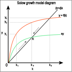
Figure 1: Solow growth model diagram (Commons.wikimedia.org, 2017)

Whether the initial ratio of labour to capital is more, then labour and output would grow slowly than capital and vice versa. This growth analysis is convergent to equilibrium path – the steady state to begin with any capital-labour ratio. Given exogenous s, n and g (rate of tech progress) and a Cobb-Douglas production function:

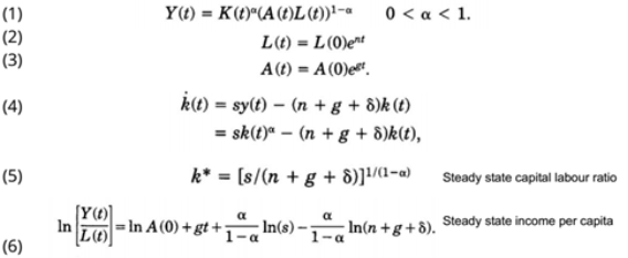
Figure 2: Solow model derivation (Weil, Mankiw and Romer, 1992)

According to Mankiw, Romer and Weil, s (savings) and n (population growth) determine steady-state level of income per capita [(f(k*)] ={(n+δ)/s} k*). Steady state capital-labour ratio related positively to rate of saving and negatively to rate of population growth. (Weil, Mankiw and Romer, 1992)

MRW paper (1992) analyses that an Augmented Solow Model which includes accumulation of human and physical capital provides an excellent definition of the cross-country data. As long as any given rate of human capital accumulation, higher s or lower n leads to higher f(k*) and thus a higher level of H*. Human capital accumulation may be correlated with s and n, leading to omitted variable bias.

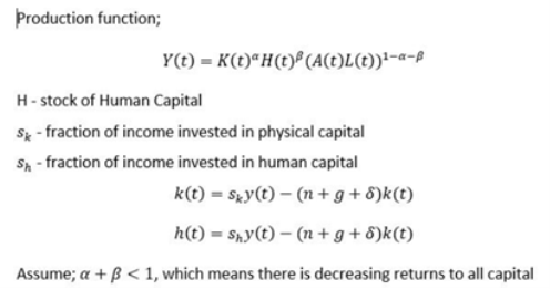
Figure 3: Production Function (Weil, Mankiw and Romer, 1992)

Using cross-country data, study finds s and n affect income in directions predicted by Solow, however; it does not correctly predict magnitude, effect on saving and income growth is large, the Solow model cannot account for international differences in income. Moreover, assumes omitted variables exist (human capital accumulation & physical capital), estimated impacts of saving and labour force growth much larger than model predicted.

Equation for income as a function of the rate of investment in physical capital, the rate of population growth and the level of human capital:

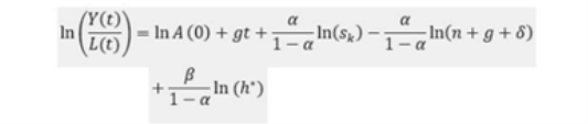
Figure 4: Equation for income (Weil, Mankiw and Romer, 1992)

The major part of the cross-country development literature that alludes to the Solow model has utilised a determination where international differences in the capital-output ratio are due to steady-state differences in output per person for a constant level of technology. The MRW paper shows that Solow model does not predict convergence and does not explain long run differences in growth rates, it predicts that income per capita in a given country converges to steady-state value of the country. (Weil, Mankiw and Romer, 1992)

The Solow growth model correctly predicts the directions of S and N, but it does not correctly predicts the magnitudes. Convergence is slower in the augmented Solow model than in the textbook Solow model. Differences in saving, education, and population growth should explain cross country variation, but it can also explain most of the international variation. Over time there will be further inclusion of other variables as well as population growth, saving and human capital which will explain the cross-country differences, for example: tax policies, education policies, tastes for children and political stability.

ANALYSIS

Empirical Analysis

Mankiw, Romer and Weil’s study explored determinants of standard of living in relation to the Solow growth model by investigating the following dimensions (Mankiw, Romer and Weil, 1992):

• Higher saving rate countries results in higher real income.
• Highly populated countries result in lower real income. (Assuming g and δ are constant across countries).

The effect of savings and population growth on real income forms the basis of the principle speculation of the Solow growth model. Recall, the computed steady state income per capita is:

where α is the capital share in income and indicates an income per capita elasticity in terms of the savings rate of approximately 0.5, and an elasticity in terms of population growth or (n + g + δ) of approximately -0.5.

One of the main assumptions here is that g – improvement with respect to technological progress, is constant across countries. As this ‘improvement’ is not country accurate it is assumed that g is constant. Another assumption is the rate of depreciation δ to be constant across countries as well mainly due to the lack of data in relation to variation of depreciation rates across countries. We will assume as value of g + n equal to 0.05, which is same assumption made by Mankiw, Romer and Weil in their paper (1992).  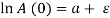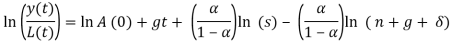In the computed steady state of income per capita equation, the term A (0) illustrates various factors such as institution, technology, resources, climate and since these factors varies across countries, we must equate it: , where corresponds to country-specific shocks and is a constant. (Mankiw, Romer and Weil, 1992) Thus, by taking the log of the computed steady state income per capita equation at a given time- t, becomes the following:

Like Mankiw, Romer and Weil, we need to assume that s and n are independent of the term . In other words, the average share of real investment in real GDP and the average population growth rate of a given country is independent to country-specific shocks. Based on this assumption, by accounting for the Ordinary Least Squares method, the values of coefficients of the fundamental equation can be estimated.

Mankiw, Romer and Weil illustrated three reasoning for the independence assumption, that is, where s and n are independent of the term . (1992) First, savings and population growth rate are considered endogenous variables in any economic growth model. Second, according to Mankiw, Romer and Weil, many economists have presented casual verdicts regarding the association between savings, income and population growth. Third, as the model speculated the value as well as the signs of the coefficients of savings and population growth, the OLS method will allow testing for salient biases.

Recall, in the right model the coefficients or elasticities of Y/L are approximately 0.5 with respect to s and approximately -0.5 with respect to (n + g + δ). Now, the joint null hypothesis for testing the model is- ‘the Solow growth model and identifying assumptions are accurate’. And the alternate joint hypothesis is- ‘the Solow growth model and the identifying assumptions are inaccurate’. If, the magnitudes of the elasticities are dissimilar to approximate values of the identifying assumption then we reject the null hypothesis. This would also mean that the Solow growth model is inaccurate and cannot account for variation in income across countries with respect to savings and population growth.

H₀ = The Solow growth model and the identifying assumptions are accurate.

H_a = The Solow growth model and the identifying assumptions are in accurate.

By running the Ordinary Least Squares method on the fundamental equation stated above, we fit a regression line that will estimate the coefficients of s and (n + g + δ).

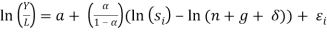
Reporting from Mankiw, Romer and Weil (1992), “conditional convergence” is an occurrence that the Solow growth model can speculate by limiting or controlling the factors of the steady state. Recall, the following equation will be used to run regression in order to determine for conditional convergence without human capital:

Data, Empirical Methodology and Definition of Variables

The data collected from the World Bank Organisation, Penn World Tables and the U.K. Data Service comprises of one dependent variable and two independent variables. The dependent variable is the “log of GDP per capita” and the independent variables are- “log of average share of real investment in real GDP” and “log of average rate of growth of the working age population (15 years – 64 years)”. The sample size is; n = 162 and the data is a cross-sectional data for the year 2007 and 1970 separately. A subsample of the data is also tested this subsample refers to the countries which form a part of the Sub-Sahara Africa region. The sample size of the subsample data is 30. (Refer to Appendix A) The following variables of the whole sample data are the following:

• Real GDP per capita for 1970 and 2007 respectively (Y/L: real GDP divided by the population in 1970 and 2007 respectively)
• Average growth rate of GDP per worker for the period 1970-2007 (Growth GDP/Worker: computed as ((GDP/Worker07)/(GDP/Worker70))^(1/37) – 1 )
• Growth rate of population during the period from 1970 to 2007 (n: computed as ((population07/population70))^(1/37) – 1 )
• Average investment share of real GDP per capita during the periods 1970 and 2007. (S_k: percentage share of real GDP per capita)

A multivariable regression examination will be carried out on the fundamental equation stated above and a restricted regression will be carried on the same equation in order to estimate the magnitudes and signs of the coefficients of s and (n + g + δ) using Ordinary Least Squares. The OLS method does this by minimizing the difference between the observed values and the speculated values which are forecasted by the linear approximation of the data. This method is used by economists and analysts to test economic models, econometric models, and hypothesis testing using real world data. (Koutun and Karabona, 2013) The software Microsoft Excel is used to run regression analysis on the data. The Excel output will comprise of a 95% lower and upper bound confidence, in addition to the standard errors (s.e.e.), adjusted R² and p-values which are of importance to us.

A restricted regression analysis will be performed on the fundamental equation. The restricted equations without human capital is the following:

  (without human capital)

In the restricted regression analysis, the mean of the F-statistics will be accounted for as this will help us gauge whether the fit of the restricted equation is notably or not notably dissimilar from the not restricted equation. We anticipate values of both the equation to be similar, thereby the equations should also be similar, and then we can conclude by not rejecting the null hypothesis. The R² is also known as the Coefficient of Determination which is a measure of the “Goodness of Fit” which describes how efficiently a model fits all the observation in a sample and can be used to predict values based on the model. The adjusted R² is useful to check whether the addition of a variable in a model is enhancing or disrupting the model. The fit ranges from 0 to 1, and the value approaching 1 indicates a good fit. (Koutun and Karabona, 2013)

The variables that are defined in Table 1 will be used in the regression analysis.

Empirical Results

One of the main principles of the neoclassical Solow growth model is that a certain country attains its steady-state level of income per capita at a point where the savings rate is higher while the population growth rates, technological growth rates and depreciation of capital rates are lower. Hence, based on this principle, from the regression estimation, the following is anticipated regarding the coefficients:

• Positive Savings Rate coefficient.
• Negative (n + g + ) coefficient.
• Values of the coefficient ln(s) and ln(n + g + δ) should be equal in magnitude and opposite in signs.

Recall, that both, the basic Solow Growth Model as well as the extended Solow Growth model are estimated by regressing the natural logarithm of real GDP per capital in 2007 to the natural logarithm of average investment share of real GDP, which is also the considered the savings rate, and the population growth rate.

The estimation outcomes of the basic Solow growth model are documented in Table 2.  Refer to Appendix B, C, D and E.

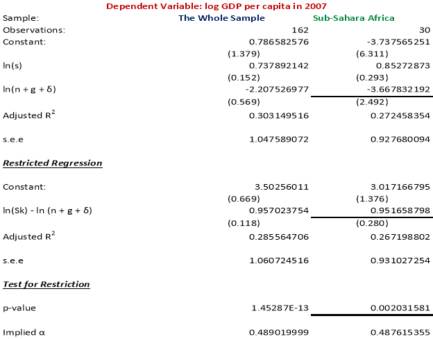
In both the samples, the coefficient of savings rate and the coefficient of the sum of population growth rates, technological advancement rates and depreciation rate have signs as anticipated. Accounting for the t-test, we also find that, in the Sub-Sahara Africa countries sample, at 5% level of significance, the savings rate that is the coefficient of ln is highly statistically significant. However, for the sample the coefficient of ln(n + g + δ) is not statistically significant. For the whole sample, both the coefficients of the estimates are not statistically significant at 5% level of significance.

In addition, as per Mankiw, Romer and Weil (1992), the coefficient of the restricted regression estimate should be equal to the coefficient of ln(s) in the unrestricted estimation, holds true for both the samples in our estimation.

An assertion made by the Solow growth model, which is that ‘differences in technology accounts for the cross-country differences in labor productivity or income per capita’ is refuted by the regression estimated for both the samples. Notice that the Adjusted R²is approximately equal to 0.303 and 0.272 for the whole sample of countries and the Sub-Sahara Africa countries respectively. The small value of the Adjusted R² suggests that the assertion made by the Solow model is contradicted, as most of differences in income per capita is explained by both the variables in this case. This small value of the coefficient of determination could also be due to the exclusion of some important variables in the sample data. In the steady state of income per capita, implied α which refers to the capital share in income has a value of 0.489 and 0.488 for the whole sample and the Sub-Sahara African countries sample respectively. These values are appreciably close to the predicted values of income per capita elasticities which is equally to 0.5 and -0.5. Hence, the model does not significantly refute the speculation that capital share in income should be approximately one third.

The regression of real GDP per capital for 2007 on average share of real investment in real GDP and population growth rate can, to a great extent, rationalize the variation in real GDP per capital i.e. income. However, as the implied α values are not significantly high as well as not equal to predicted value of being equal to one third i.e. 0.33, one cannot conclusively conclude that the basic Solow growth model is highly successful.

Absolute Convergence Model:

According to the convergence theory the per capita income of richer economies is likely to grow at a slower rate in comparison poorer countries. This phenomenon can be attributed to the strength of the capital diminishing returns which is stronger in developing countries, like Brazil, India, Senegal and Mexico, in comparison to developed countries like Canada, Denmark, France, New Zealand and Australia. Based on this model, income is most likely to be negatively related with growth in income at time zero during the period of the sample, 1970-2007. We anticipate the sign of the logarithm of real GDP per worker to be negative and a high regression coefficient.

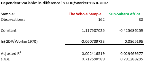Table 3: Test for Absolute Convergence. Refer to Appendix F and G

The coefficient of the natural logarithm of income per worker for the whole sample has a negative sign as predicted, which is support of the convergence theory, however, in the Sub-Sahara countries sample, is does not have negative sign, in contradiction to the convergence theory. The positive coefficient of the income per worker variable for Sub-Sahara countries could also indicate while doing the test of the convergence theory, the sample needs to include some developed countries, unlike the sample of Sub-Sahara countries, in which most of the countries are either developing or underdeveloped, the support for the convergence theory cannot be tested entirely using this sample of countries. In addition, the low coefficient value of the whole sample, that is, -0.0607 also suggests that this value is not entirely statistically significant. The coefficient of determination is low in both the sample, which also indicates a weak goodness of fit for this estimation.

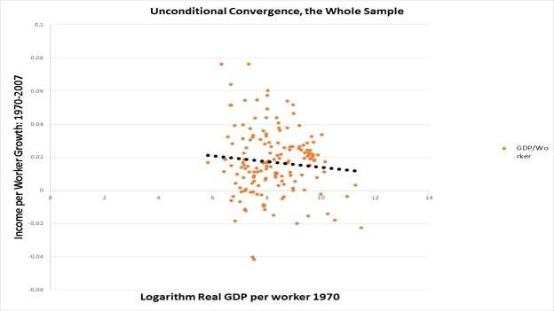Graph 1: Unconditional Convergence, the Whole Sample.

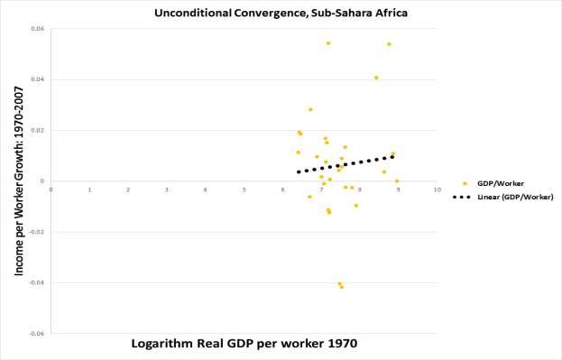Graph 2: Unconditional Convergence, Sub-Sahara Africa

In Graph 1 and Graph 2, the x-axis represents the logarithm of real GDP per worker in 1970 while the y-axis represents the growth in income per worker during the period 1970-2007. The graphs are plotted to indicate the existence or non-existence of unconditional convergence in the whole sample of countries and the countries in the Sub-Sahara Africa sample countries. To conclude the presence of unconditional convergence we anticipate a downward-slopping trend line from left to right. Graph 1 exhibits a downward slopping trend line indicated by the black solid-dotted line which is support of the presence of convergence in the sample of countries. However, Graph 2, exhibited an upward slopping line, which is against the convergence theory.

Conditional Convergence: Without Human Capital

The regression coefficients are estimated by reviewing the equation (1.2); we regress the difference in the logarithm of real GDP per capita during the period 1970 to 2007 on the logarithm of real GDP per capita in 1970, also considering the savings rate and the population growth rate in the equation.  The sign of the coefficients is as anticipated- the savings coefficient is positive while the population growth coefficient is negative. The coefficients of the income level in 1970, the savings rate and the population growth rate are significant for both the samples.

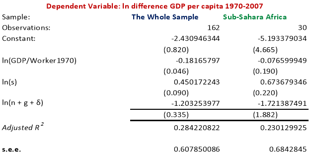Table 4: Test for Conditional Convergence without human capital. Refer to Appendix H and I.

In absolute values, the coefficient on population growth rate is greater than the coefficient on savings rate, indicating that the lower income per capita needs to spread over a larger population thereby reducing income per capita itself.

Conclusion

Under the principle of neoclassical Solow growth model, the regression estimation of the whole sample and Sub-Sahara we found that at 5% level of significance, the coefficient of ln(s) is highly significant while ln(n + g + δ) is not significant in Sub-Sahara and in whole sample, coefficients are both not significant. The small value of Adjusted R² states the assertion of Solow model is contradicted. Additionally, in the steady state of income per capita, implied α which is closed to the predicted value indicate the model does not strongly contradict the speculation that capital share in income is approximately equal to 1/3. Although the regression of real GDP in 2007 rationalizes the variance, the hypothesis, the basic Solow model which is significant successful cannot be verified because of implied α. With regard to convergence, based on convergence theory, we calculate the logarithm of real GDP per worker. The whole sample supports the convergence while Sub-Sahara rejects the convergence. However, the coefficient of the whole sample which is low indicates the value of coefficient is not significant. Under unconditional convergence graph, the coefficient prove the weak goodness of fit for estimation. Setting a condition of convergence, which is without human capital, the coefficients of the income level in 1970, the savings rate and the population growth rate are significant.

Word Number: 3281

Bibliography

• Commons.wikimedia.org. (2017). File:Solow growth model1.png – Wikimedia Commons. [online] Available at: https://commons.wikimedia.org/wiki/File:Solow_growth_model1.png [Last Accessed 20 Mar. 2017].
• Koutun, Alina and Patrick Karabona. “An Empirical Study Of The Solow Growth Model”. MALARDALENS HOGSKOLA ESKILSTUNA VASTERAS. N.p., 2013. Web. [Last Accessed 9 Mar. 2017].
• Mankiw, G. N., Romer, D., & Weil, D. N. (1992, May). A Contribution to the Empirics of Economic Growth. The Quarterly Journal of Economics, 107(2), 407-437
• Solow, R. (1970). Growth theory: an exposition. 1st ed. Oxford: Clarendon, pp.

Appendix A:

Appendix B: Regression, the Whole Sample

Appendix C: Restricted Regression, the Whole Sample

Appendix D: Regression, Sub-Sahara Africa

Appendix E: Restricted Regression, Sub-Sahara Africa

Appendix F: Unconditional Convergence Test, the Whole Sample

Appendix G: Unconditional Convergence Test, Sub-Sahara Africa

Appendix H: Conditional Convergence Test, the Whole Sample

Appendix I: Conditional Convergence Test, Sub-Sahara Africa