Cumulative Prospect Theory: Vietnamese Market

After the invention of Cumulative Prospect Theory, many research have been conducted in attempt to test the assumption of the theory and also measure its parameters by analyzing empirical data, i.e. the α, β shaping the convexity or concavity of the utility function, the loss aversion index λ determining the utility function’s slope in the loss region and δ, γ which define how people distorts probabilities when dealing with a choice problem.

This chapter we will discuss and review former result involving estimating the parameters. The results of the research will be tested under a set of data in Vietnamese market in chapter 3.

1. Tversky and Kahneman (1992)

Apart from the suggestion of the prominent argument of Cumulative Prospect Theory, Tversky and Kahneman also conducted an experiment to estimate the parameters of the utility function as well the weighting function. Particularly, they recruited 25 students from Berkeley and Stanford who had no training in decision making before the time. Each one of the subjects participated in 3 separate sessions that were organized several days apart.

In the experiments, a computer displayed a prospect with outcomes and probabilities and its expected value. The computer also displayed seven certain outcomes which were placed within two extreme outcomes of the prospect. The subjects were asked to show their preference between each of the seven sure outcomes and the initial prospect.

To refine the certain equivalent of the prospect they continued to reduce the scope of the certain value. They displayed another set of seven certain outcomes which were placed linearly within the highest certain outcome rejected (the outcome is less preferred than the prospect) and the lowest certain outcome accepted (which is more preferred than the prospect). The subjects showed their preference secondly. The certain equivalent of the prospect was defined as the middle point of the highest outcome rejected and the lowest outcome accepted in the second set of sure outcomes. During the experiment, the computer monitored the consistency among the subjects’ answers, every error or biases were automatically rejected.

Because Cumulative Prospect Theory is a very complex choice model, the estimation could become really problematic. If the form of the theory’s functions are allowed to be flexible, the number of parametric estimations will be too large. Therefore, in the study, Tversky and Kahneman assumed the value function with the piecewise power form and the weighting function with the formula:

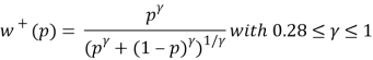
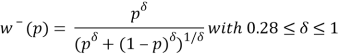
Then they conducted a nonlinear regression to estimate the parameters contained in the equation above separately for each subject. They found that the exponent of the value function is 0,88 for both gain side and loss side, satisfying the diminishing sensitivity assumption and therefore presenting an S-shape value function. The loss aversion index λ = 2,25 indicating loss aversion phenomenon. For the weighting function, γ and δ were estimated to be respectively 0,61 and 0,69 satisfying the condition that the weighting functions are increasing.

2. The trade-off method of Fennema and Van Assen (1998)

The aim of this work is to investigate the shape of value function. Generally, from behavioral point of view, the utility for loss must be convex rather than concave. Most empirical measurement reinforced the statement. However, the measurement employed methods that are either biased by certainty effect or necessitate very complex parametrical estimations. In this paper, Fennema and Van Assen proposed a new approach to measure the parameter, the trade-off method. The result is that they find out a utility function fitting with the assumption of Cumulativ Prospect Theory.

In the experimental, 64 students from University of Nijmegen are recruited to be subjects. Most of them were majoring in psychology. The subjects participated in 2 separate sessions of the experiment.

The subjects’ task is to choose between two prospects (see Figure 2.1) that are both defined on the same events E₁ (upper branch) and E₂ (lower branch) having probabilities p₁ (for example, equal to 1/3) and p₂ (therefore, being 2/3) respectively. If event E₁ occurs, the right prospect yields more money than the left (an additional $500 in the example). If E₂ occurs, the left prospect yields a smaller loss than the right. So, the task for the subject is essentially to make a tradeoff: does the extra money that the right prospect yields in case of E₁ outweigh the smaller loss that the left prospect yields in case of E2? The experiment was the outward trade-off for loss. The inward one is to be set with E₁ of the right prospect smaller than E₁ of the left prospect so that the preference switching point is bigger than E₂ of the left prospect.

Turn back the example, the free value (labelled ‘?’ in Figure 2.1) is varied in order to find the preference switching point. For example, if the free value is -$26, the possibility of losing one additional dollar (if one chooses the right prospect) in case E₂ occurs can be easily outweighed by the chance of receiving an additional $500 if E₁ occurs. If the additional loss of the right prospect in event E₂ is increased, at some point the trade-off will turn in favor of the left prospect. For example, the preference switching point where the subject is indifferent between the left and right prospect lies at the value of -$60. This gave an information that the objective values of the two prospects are the same, or:

The authors continued to ask the subject to do the same experiment with another couple of prospect as follows:

Assuming the result showed that the switching point labelled “?” is -$100. For given, they obtained another equation:

Combining the two equations above and dropping the factor , they gained the following result:

Through this indifference equation, we can see that the distorted probability does not matter in the method. A series of the experiment was conducted and this procedure is chained, in the sense that a response of a question is used as an input for the next question. This procedure yielded several indifference equations like this. These equations were the input for a nonlinear regression with the utility function formed by the piecewise power formula Tversky and Kahneman (1992) had suggested.

The result of the regression, they induced an estimation of the exponents of value function, σ = 0,39 and β = 0,84. These result present the convex utility for loss side and concave utility for gain side. Their finding of convex utilities for losses shows that utility measurement is primarily responsive to diminishing sensitivity. This also reinforces the view that utilities are the result of a constructive process: diminishing sensitivity has nothing to do with people’s evaluation of money but is purely a matter of perception of numbers. To interpret the functions that result from responses that are predominantly determined by diminishing sensitivity as utility functions goes a long way from the interpretation that Cramer, Bernoulli, and Bentham had in mind. It shows once again that in predicting and aiding individual decision behavior, it is important to know the precise presentation of the decision problem, and the psychological mechanisms that govern its perception.

3. The traceable method of Abdellaoui (2007)

In the paper, Abdelaoui introduced the elicitation method. The elicitation method comprises of three stages. In the first stage utility is elicited on the gain domain, in the second stage utility is elicited on the loss domain, and in the third stage the utility on the gain domain and on the loss domain are linked. All measurements are based on the elicitation of certainty equivalents for two-outcome prospects. The certainty equivalents of different elicitation questions are not chained. This has the advantage that error propagation does not affect our findings.

We assumed that the observable utility U in prospect theory is a composition of a loss aversion coefficient λ > 0, reflecting the different processing of gains and losses, and a basic utility u that reflects the intrinsic value of outcomes for the agent. This decomposition was also adopted by Tversky and Kahneman (1992), Shalev (2000), and Bleichrodt, Pinto, and Wakker (2001). Formally, this assumption means that

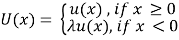
The exact definition of loss aversion depends on the specification of u. We will return to this issue later.

Consider first the elicitation of utility on the gain domain. We start by selecting a probability pg that is kept fixed throughout the elicitation of the utility function on the gains domain. They chose a series of prospects (x_i, p_g; y_i), for which x_i > y_i ≥ 0, i = 1, …, k and elicit their certainty equivalents G_i defined as follows:

Or

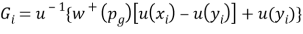
The advantage of keeping the probability p_g fixed is that only one point of the probability weighting function plays a role in the process of utility elicitation. The probability weight δ­⁺ can just be taken to be one additional parameter that has to be estimated in the utility elicitation exercise. In fact, if we adopt a parametric specification for utility, then G_i can easily be estimated through nonlinear regression. In the experiment described below we adopted the most widely used parametric specification, the power function u(x) = x^α. Thereby,

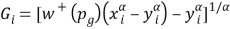
where α and are parameters being estimated.

The procedure to elicit the utility on the domain of losses is largely similar to the procedure described above for gains. We select pl = 1 − pg and a series of prospects (x_i, p_l, y_i) for which 0 ≥ y_i > x_i, i = 1,…,k and elicit their certainty equivalents L_i. The reason we set p_l = 1−p_g is that this equality is crucial in the estimation of loss aversion.

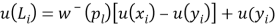
Then

In terms of measuring the loss aversion, the third stage of the elicitation procedure serves to establish the link between the utility for gains and the utility for losses and, hence, measures the loss aversion coefficient λ. This can be done through the elicitation of a single indifference. Select a gain G* from within (0,x_k], the interval for which u was determined in the first stage and determine the loss L* for which (G*, p_g; L*) ~ 0.

The is easily estimated because , , , are both determined above.

In the experiment, they recruited 48 graduate students in economics and mathematics at the Ecole Normale Supérieure, Antenne de Bretagne, France. The experiment was run on a computer. Responses were collected in personal interview sessions. Subjects were told that there were no right or wrong answers and that they were allowed to take a break at any time during the session. The responses were entered into 17 the computer by the interviewer, so that the subjects could focus on the questions. Before the experiment started subjects were given several practice questions. The experiment lasted 60 minutes on average, including 15 minutes for explanation of the tasks and practice questions.

All indifferences were elicited through a series of binary choices. Each binary choice corresponded to an iteration in a bisection process. After each choice the subject was asked to confirm his choice. The author used a choice-based elicitation procedure because previous studies have found that inferring indifferences from a series of choices leads to fewer inconsistencies than asking subjects directly for their indifference values (Bostic, Herrnstein, and Luce 1990). In each choice a subject was faced with two prospects, labeled A and B, where prospect A was always riskless. Prospects were displayed as pie charts with the sizes of the slices of the pie corresponding to the probabilities.

Six certainty equivalence questions were used to elicit the utility function for gains and 6 certainty equivalence questions to elicit the utility function for losses. The prospects for which the certainty equivalents are determined are displayed as follows:

Substantial money amounts are used to be able to detect curvature of utility; for small amounts utility is approximately linear (Wakker and Deneffe 1996). The author used round money amounts, multiples of €1000, to facilitate the task for the subjects. As shown by the table, the measurements were not chained and, hence, not vulnerable to error propagation.

The elicitation method also allows examining the validity of prospect theory with utility under the power form. As a first test, the researcher elicited the certainty equivalents for two different values of p_g, p_g = 1/2 and p_g =2/3 and, consequently, p_l =1/2 and p_l = 1/3 for losses. Under prospect theory he observed no systematic differences between the utility elicited with p_g =1/2 and the utility elicited with p_g = 2/3. For losses no difference should be observed between the utility elicited with p_l = 1/2 and the utility elicited with p_l = â…“.

The order in which the 24 certainty equivalents were elicited was random. At the end of the elicitation of the utility for gains and the elicitation for losses the research repeated the third iteration for eight questions, four for gains (two for p_g = 1/2 and two for p_g = 2/3) and four for losses (two for p_l = 1/2 and two for p_l = 1/3). The questions that were repeated were determined randomly. To determine the loss aversion coefficients, the author selected G*1,…,G*6 and determined L*j such that (G*j , 0,5; L*j ) ~ 0, j = 1,…,6. The method only needs one indifference to elicit the loss aversion coefficient λ. They used 6 questions to have another test of the validity of prospect theory with (3). Under prospect theory with (3), the 6 values of the loss aversion coefficients that are observed should be equal. The order in which these questions were asked was random. They repeated the third iteration of two randomly determined questions to test for consistency.

The result of the experiment is that α = 0.86, β =1,06 and λ = 2,61, in addition, w⁺(½) = 0,46; w⁺(â…”) = 0.53; w⁻(â…“) = 0.34 and w⁻ (½) = 0,45 . The research found concave utility for gains, strong evidence for loss aversion, and data on probability weighting which were consistent with inverse S-shaped probability weighting. However, the experiment found no evidence on the convexity of utility function for loss.