Analysis of Optimal Conditional Heteroskedasticity Model

Abstract:

Recently cryptocurrency markets have seen an immense growth. Bitcoin is one of the most popular cryptocurrencies accounting for the highest share of all cryptocurrency markets, even though it still remains rather unclear whether it resembles more to a currency, a commodity or an asset. Previous research has shown that Bitcoin is often used for investment purposes, a fact that suggests the importance of analysing its volatility. In this article, we examine the optimal conditional heteroskedasticity model, not only in terms of goodness-of-fit, but also in terms of forecasting performance, an area which has been underexplored in the case of Bitcoin. According to the results, the optimal conditional heteroskedasticity model that can fit the series is not the same as the one that can forecast it better. As modelling GARCH effects in Bitcoin market effectively is crucial for appropriate portfolio management, our results can help investors and other decision makers make more informed decisions.

Keywords: Bitcoin, Cryptocurrencies, GARCH, Volatility, Forecasting

JEL classification: C22, C5, G1

1. Introduction

Over the last few years, the analysis of Bitcoin has drawn a lot of both public and academic attention. Bitcoin is the first implementation of a concept called “cryptocurrency”, which was first described in 1998 by Wei Dai on the cypherpunks mailing list, suggesting the idea of a new form of money that uses cryptography to control its creation and transactions, rather than a central authority, but the first Bitcoin specification was published in 2009 in a cryptography mailing list by Satoshi Nakamoto (Bitcoin.org 2017).

The market of cryptocurrencies has grown remarkably with Bitcoin being considered the most famous cryptocurrency, with an estimated market capitalisation of $19.6 billion (coinmarketcap.com accessed on 8th March 2017), which currently accounts for around 84.4% of the total estimated cryptocurrency capitalisation. An overview of Bitcoin can be found in, e.g., Becker et al. (2013), Dwyer (2015), Frisby (2014), Böhme et al. (2015) and Selgin (2015). Hence, Bitcoin is only briefly introduced here.

It has been previously argued that Bitcoin shares some elements of currencies. However, recent fluctuations in Bitcoin prices (see Figure 1) have resulted in unpredictable volatility undermining the role Bitcoin plays as a unit of account (Cheah and Fry 2015), while users have adopted Bitcoin not only as a currency but also for investment purposes. In fact, new users tend to trade Bitcoin on a speculative investment intention basis and have low intention to rely on the underlying network as means for paying goods or services (Glaser et al. 2014). The Bitcoin market is thus highly speculative at present, and therefore Bitcoin may be mostly used as an asset rather than a currency (Baek and Elbeck 2015; Dyhrberg 2016a).

Moreover, recent studies have examined the hedging capabilities of the Bitcoin (see, e.g., Dyhrberg (2016a, b), justifying the view of it as an asset, as well as the role of different exchanges in the price discovery process of Bitcoin (Brandvold et al. 2015), while it has also been previously shown that cryptocurrency markets share some stylised empirical facts with other markets, e.g., a vulnerability to speculative bubbles (Cheah and Fry 2015). Consequently, Bitcoin has a place in the financial markets and in portfolio management (Dyhrberg 2016a).

Bitcoin has posed great challenges and opportunities for policy makers, economists, entrepreneurs, and consumers since its introduction (Dyhrberg 2016b), while Bitcoin price volatility seems to be a major concern for most of the general public at this time (Bouoiyour and Selmi 2016). As a result, studying Bitcoin price volatility is of high importance.

Following the extensive literature on modelling financial asset prices using the family of Generalised Autoregressive Conditional Heteroskedasticity (GARCH) models, recently there has also been an increased interest in modelling Bitcoin price volatility using similar methods. Previous studies have used different types of GARCH models when examining the Bitcoin price volatility.For example, the simple GARCH model has been employed by Glaser et al. (2014), Gronwald (2014) and Dyhrberg (2016a). On the other hand, other studies have considered extensions to the GARCH model in order to study asymmetries in Bitcoin price volatility. For instance, the Exponential GARCH (EGARCH) model has been used by Dyhrberg (2016a) and Bouoiyour and Selmi (2015, 2016), the Threshold GARCH (TGARCH) (GJR-GARCH) model has been employed by Dyhrberg (2016b), Bouoiyour and Selmi (2015, 2016) and Bouri et al. (2017), while the Asymmetric Power ARCH (APARCH) and Component with Multiple Threshold-GARCH (CMT-GARCH) models have been used by Bouoiyour and Selmi (2015, 2016).

Nevertheless, it is rather unclear which conditional heteroskedasticity model should be used when studying the Bitcoin price volatility. Previous studies of the Bitcoin price volatility have focused mainly on the use of a single conditional heteroskedasticity model, without comparing different GARCH-type models, though, with the only exceptions being the studies of Bouoiyour and Selmi (2015, 2016), which have split[PK1] the sample into different sub-periods, though, and the study of Katsiampa (2017/forthcomng?), which has not considered the risk-return relationships, though[PK2]. In addition, little attention has been paid to forecasting the volatility of the Bitcoin prices. To the best of the author’s knowledge only the study of Bouoiyour and Selmi (2016) has examined the forecasting performance of the CMT-GARCH and APARCH models, but no study has compared the predictive ability of different GARCH models with regards to Bitcoin. Consequently, we aim to contribute to the literature by investigating which conditional heteroskedasticity model can describe and forecast the Bitcoin prices better.

The remainder of the article is organised as follows: The next section presents the models employed in this study. The data and methodology used in the study are discussed in the third section, while the fourth section details our empirical results. Finally, the conclusions drawn and the implications are presented in section five.

2. Models

In this section, the models used in this research are introduced. The models consist of an Autoregressive model for the conditional mean and a first-order GARCH-type or a GARCH-in-Mean-type model for the conditional variance[1], as follows

,

, ,

where is the Bitcoin price return on day , is the error term, is a white noise process, is the conditional standard deviation, and hence is the conditional variance. When is equal to zero, the resulting model is the autoregressive model with a GARCH-type specification for the conditional variance, while when is different from zero a GARCH-in-Mean-type specification for the conditional variance is obtained. Adding the standard deviation to the mean equation measures the risk and helps with the identification and measurement of any risk-return relationship.

The conventional GARCH(1,1) model is represented by

,

with , and . The GARCH model (Bollerslev 1986) is undoubtedly one of the most popular models for describing the conditional variance of financial returns. Nevertheless, since its introduction, there have been proposed many extensions of the GARCH model and there have been a lot of advances in modelling the conditional variance. Hence in this study, we also consider five extensions to the linear GARCH model, namely the EGARCH model of Nelson (1991), the TGARCH model introduced by Glosten et al. (1993), the APARCH model proposed by Ding et al. (1993), the Component GARCH (CGARCH) model of Engle and Lee (1999) and the Asymmetric CGARCH (ACGARCH) model. All these models constitute examples of extensions of the simple GARCH model and have attempted to describe the conditional variance more accurately. Moreover, compared with the simple GARCH model, the EGARCH, TGARCH and APARCH models allow for different volatility responses to opposite signs of the previous shocks.

More specifically, the EGARCH model is defined as

,

and considers the asymmetric volatility responses to negative news, that is , and positive news, , as given by the sign of , if is different from zero.

The TGARCH model is given by

,

where is the indicator function, with if and 0 otherwise, suggesting that positive shocks and negative shocks have again different effects on the volatility, if is different from 0.

On the other hand, the APARCH model is defined as

,

where , ,, and . This model imposes a Box-Cox power transformation of the conditional standard deviation process and the asymmetric absolute residuals (Ding et al. 1993).

Furthermore, in contrast with the GARCH model, the conditional variance of which shows mean reversion to , which is a constant for all time, the CGARCH model allows for both a long-run component of conditional variance, , which is time varying and slowly mean-reverting, and a short-run component, , and is defined as

.

Christoffersen et al. (2008) demonstrated that by including both a short-run and a long-run component allows the CGARCH model to outperform the GARCH model.

Finally, the Asymmetric Component GARCH (ACGARCH) model combines the CGARCH model with the TGARCH model, introducing asymmetric effects in the transitory equation, and takes the following form

,

where is a dummy variable which indicates negative shocks, while positive values of suggest the presence of transitory leverage effects in the conditional variance.

3. Data and methodology

The data consists of daily closing prices for the Bitcoin Coindesk Index from 19^th July 2010 to 10^th January 2017. The estimation sample covers the period between 19^th July 2017 and 31^st December 2017 leading to a total number of 2357 observations, while the remaining ten observations are used in the forecasting sample. The Bitcoin CoinDesk Index is listed in USD and the data are publicly available online at http://www.coindesk.com/price.

The data are converted to natural logarithms, and then the returns are defined as

,

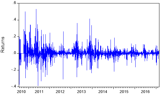
where is the logarithmic Bitcoin price index change and is the daily Bitcoin price index on day . Figures 1 and 2 illustrate the Bitcoin prices and price returns, respectively, in the estimation period.

We start the empirical analysis by producing descriptive statistics for the Bitcoin price returns, while the Augmented Dickey-Fuller (ADF) and Phillips-Perron (PP) unit-root tests are also performed to examine the stationarity of the returns. As will be seen in the next section, the results show that the series is stationary.

In order to choose the best model in terms of fitting to data, three information criteria, namely Akaike (AIC), Bayesian (BIC) and Hannan-Quinn (HQ), are employed. For given data sets, all of these information criteria consider both how good the fitting of the model is and how many parameters there are in the model, rewarding a better fitting and penalising an increased number of parameters. The preferred model is the one with the respective minimum criterion value.

However, since model selection is often not only based on a model’s goodness-of-fit to data, but also on forecasting performance, it is important to also check the models’ predictive ability, as a better fitting model does not always lead to better forecasts. Hence, the best model specification in terms of forecasting is selected according to the Root Mean Squared Forecasting Error (RMSE), Mean Absolute Forecasting Error (MAE) and Mean Absolute Percentage Forecasting Error (MAPE), all of which are used as measures of forecasting performance. Although the RMSE is one of the most commonly used measures of predictive ability, the additional measures have been used in order to verify the results.[2] The models’ forecasting performance is evaluated based on out-of-sample forecasts, and model selection is examined in terms of both multi-step-ahead and multiple 1-step-ahead forecasting. The preferred model is the one with the lowest values of the measures of predictive ability.

Fig. 1. Daily closing prices of the Coindesk Bitcoin Index (US Dollars).

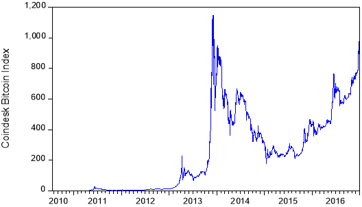
Fig. 2. Daily Bitcoin price returns.

4. Results

Table 1 reports the descriptive statistics for the daily returns of the Bitcoin price index. The daily average closing return is positive and equal to 0.5805% with a standard deviation of 0.0606. Moreover, the returns are positively skewed, indicating that it is more likely to observe large positive returns, and leptokurtic as a result of significant excess kurtosis. The Jarque-Bera (JB) test confirms the departure from normality, while the results of the ARCH(5) test for conditional heteroskedasticity show evidence of ARCH effects in the returns of the Bitcoin price index. Therefore the Autoregressive model for the conditional mean needs to be combined with an Autoregressive Conditional Heteroskedasticity process to model the conditional variance. It can be noticed that the ARCH effects can also be observed from Figure 2 where large (small) price changes tend to be followed by large (small) price changes over time. Furthermore, the results from both the Augmented Dickey-Fuller and Phillips-Perron unit root tests indicate that stationarity is ensured.

Table 1. Descriptive statistics and unit roots tests.

Note: *** indicates the rejection of the null hypotheses at the 1% level.

Next, the estimation results of the GARCH-type models are discussed. The conditional mean equation includes a constant and an autoregressive term, while the conditional variance is modelled by various competing GARCH models. The model parameters are estimated by using the maximum likelihood approach under the Gaussian distribution.

Table 2 presents the estimation results of each model. These include the model parameter estimates, the log-likelihood values and the three information criteria values. In addition, the ARCH(5) test to check whether the conditional heteroskedasticity is eliminated and the Ljung-Box test for autocorrelation with 10 lags applied to squared residuals, as well as the Jarque-Bera (JB) test of normality of the residuals have been used as diagnostic tests, the results of which are also reported in Table 2.

According to the results, both the AIC and HQ information criteria select the AR(1)-ACGARCH(1,1) model as the preferred model in terms of fitting to data, followed by the AR(1)-CGARCH(1,1)-M and AR(1)-CGARCH(1,1) models, suggesting the important role of having both long-run and short-run components of conditional variance. The log-likelihood is also maximised under the AR(1)-ACGARCH(1,1) model. On the other hand, the preferred model according to the BIC is the AR(1)-CGARCH(1,1), followed by the AR(1)-ACGARCH(1,1) model. The latter result could be explained, though, by the fact that the BIC penalises more a higher number of model parameters, and hence the selection of the AR(1)-ACGARCH(1,1) model seems appropriate.

It can also be noticed that for the AR(1)-ACGARCH(1,1) model all the parameter estimates are statistically significant. Moreover, the results of the ARCH(5) and tests applied to the squared residuals of the AR(1)-ACGARCH(1,1) model indicate that the selected AR(1)-ACGARCH(1,1) model with Gaussian distribution is correctly specified because the hypotheses of no remaining ARCH effects and no autocorrelation cannot be rejected. Furthermore, despite the fact that the residuals still depart from normality, the value of the Jarque-Bera statistic associated with the residuals of the AR(1)-ACGARCH(1,1) model is much lower than the corresponding value for the raw returns.

Consequently, the AR-ACGARCH model seems to be useful to describe the volatility of the returns of the Bitcoin price index. This result seems to be consistent with the study of Bouoiyour and Selmi (2016)[PK3] who found that the best model for the period from December 2010 to December 2014 is the CMT-GARCH model, which also includes both transitory and permanent components as well as thresholds related to positive and negative shocks.

With regards to the out-of-sample forecasting performance, the five- and ten-day-ahead forecasts as well as the five and ten 1-day-ahead forecasts of the twelve competing GARCH-type models were generated. We then compared the models’ forecasting performance based on the three mean loss functions (RMSE, MAE and MAPE).

Table 3 reports the obtained results, while the bold numbers indicate the best model in terms of forecast accuracy. An interesting finding is that overall the information criteria for model selection in terms of goodness-of-fit do not agree with the measures of predictive ability. Even though the minimum RMSE values of the 10-step-ahead and ten 1-step-ahead forecasts were both given for the AR-CGARCH model, a result which is consistent with the Bayesian Information Criterion, the results of the other two measures of predictive ability (MAE and MAPE) showed that there are other models that perform better than the AR-ACGARCH and AR-CGARCH models when it comes to forecasting.

More specifically, the minimum RMSE values of the 5-step-ahead and five 1-step-ahead forecasts were both given for the AR-EGARCH-M model. On the other hand, the lowest MAE and MAPE values of the 5- and 10-step-ahead forecasting as well as those of the five 1-step-ahead forecasting were all given for the AR-EGARCH model. The lowest MAE value of the ten 1-step-ahead forecasting was also given for the AR-EGARCH model, while the lowest MAPE value of the ten 1-step-ahead forecasting was given for the AR-APARCH-M model.

In summary, according to our estimation results the AR-ACGARCH model is preferred to the other competing models in terms of volatility estimates for the returns. However, the preferred model in terms of forecasting is overall the AR-EGARCH. This result is crucial for portfolio management and decision making in general by individuals who use Bitcoin for speculative purposes.

Finally, it should be noted that the model parameters were estimated under the Student-t and GED distributions as well, but as there was no improvement in either the goodness-of-fit or forecasting performance, the results are not reported here.[3] This is in contrast with the results of the study of Bouri et al. (2017) who found that the TGARCH(1,1) model under the GED density is the best fit.

5. Conclusions

Over the last few years cryptocurrency markets have grown to a great extent, with Bitcoin having attracted a lot of attention from both the public and researchers. This article aimed to offer a discussion into Bitcoin price volatility by selecting an optimal GARCH-type model in terms of both goodness-of-fit to data and forecasting performance chosen among several extensions. It was found that even though the best model in terms of goodness-of-fit is the AR-ACGARCH, a result which is consistent with previous studies[PK4], with regards to forecasting performance the best model seems to be overall the AR-EGARCH. Consequently, if the objective is to find the best model in terms of predictive ability, model selection based on information criteria only might not be adequate.

As Bitcoin can combine some of the advantages of both commodities and currencies in the financial markets (Dyhrberg 2016a), it can be a useful tool for portfolio analysis and risk management. Hence, individuals in portfolio and risk management need to get a more detailed view of the Bitcoin price volatility. Our results may thus have important implications mainly for investors but also for other decision makers, such as policymakers, as they can enable them to make more informed decisions.