Algorithm to Prevent Obstacle Collision
| ✅ Paper Type: Free Essay | ✅ Subject: Computer Science |
| ✅ Wordcount: 2072 words | ✅ Published: 22 Jun 2018 |
Description: In this paper, we develop an algorithm to prevent collision with obstacles autonomous mobile robot based on visual observation of obstacles. The input to the algorithm is fed a sequence of images recorded by a camera on the robot B21R in motion. The information is then extracted from the optical flow image sequence to be used in the navigation algorithm. Optical flow provides important information about the state of the environment around the robot, such as the disposition of the obstacles, the place of the robot, the time to collision and depth.
The strategy is to estimate the number of points of the obstacles on the left and right side of the frame, this method allows the robot to move without colliding with obstacles. The reliability of the algorithm is confirmed by some examples.
Keywords: optical flow, the strategy of balance, focus of expansion, the time for communication, avoiding obstacles.
1. Introduction
The term is used for visual navigation of robot motion control based on analysis of data collected by visual sensors. Golf visual navigation is of particular importance is mainly due to the vast amount of recorded video sensor materials.
The aim of our work is to develop algorithms that will be used for the visual navigation of autonomous mobile robot. The input consists of a sequence of images that are constantly available navigation system while driving the robot. This sequence of images is provided by monocular vision system.
Then, the robot tries to understand their environment to extract data from a sequence of image data, in this case, optical, and then uses this information as a guide for the movement. The strategy adopted to avoid collisions with obstacles during movement – a balance between the right and left optical flow vectors.
The test mobile robot models RWI-B21R. The robot is equipped with WATEC LCL-902 camera (see. Fig. 1). Visuals caught using Matrox Imaging cards at a rate of 30 frames per second.

Fig. 1 – The robot and the camera.
Fig. 2 shows a flowchart of navigation.

Fig. 2 – Algorithm for prevention of obstacles.
The first optical flow vectors are computed from image sequences. To make a decision about the orientation of the robot, the calculation of the position of the image plane in the DMZ is necessary because the control is transferred to the law with respect to the focus of expansion. Then, the depth map calculates the distance to an obstacle, to provide an immediate response to a short distance from the obstacle, or to give a signal to the robot to ignore obstacles.
2. Otsenka movement
Movement in the sequence of images obtained by camera induced movement of objects in 3-D scene and / or camera motion. 3-D objects and the camera motion is a 2-D motion image plane via the projection system. It is a 2-D movements, also called apparent motion or optical flow, and should be the starting point of the intensity and color information of the video.
Most of the existing methods of valuation movements are divided into four categories: basic techniques of correlation, the basic methods of energy, basic methods of parametric model and the basic methods of differentiation. We chose the technique of differentiation, based on the intensity of the preservation of a moving point for the calculation of the optical flow, for this purpose, the standard method of Horn and Schunck (Horn and Schunck manual, B., 1981).
After calculating the optical flow, we use it for navigation solutions, such as trying to balance the number of left and right sides of the flow to avoid obstacles.
3. The laws of optical flow and management
As well as the observation point moves through the environment, and the sample beam, reflecting this point varies continuously generates an optical flow. . One way in which the robot may use this information to a movement to achieve a certain type of flow. For example, to maintain the orientation of the environment, the type of optical flow does not flow at all requests. If some flow is detected, the robot should change their strength by producing their effectors (whether wings, wheels or legs). so as to minimize this flow, in accordance with the control law (Andrea, PD; William H. & Lelise PK, 1998) ..

Thus, the change of the internal forces of the robot (as against external forces such as wind) is a function of changes in the optical flow (here from a lack of flow to the minimum flow) .. The optical flow contains information about the location of the surface and the direction of the observation point called the focus of expansion (CLE), the time to contact (TTC), and depth.
3.1. The focus of expansion (RF)
For the translational movement of the camera, the motion picture is always directed away from the only point of the corresponding projection of the vector transmission to the image plane. This point is called Focus Expansion (DF), it is calculated on the basis of the principle that the flux vectors are oriented in certain directions with respect to the focus of expansion.
At full optical flow is the horizontal part of the DF horizontally located, in accordance with the situation in which the majority of the horizontal components of variance (Negahdaripour, S. & Horn, CP 1989). It can be estimated using a simple counting method, which counts the horizontal components of the signs, which focus on each point of the image. At the point where the maximum divergence, the difference between the number of RF components on the left of the right and the number of components must be minimized. Similarly, we can appreciate the vertical position of the FF by identifying the positions of most of the vertical components.

Fig. 3 – Calculation of the DF.
Fig. 4 shows the result of calculating the risk factors in indoor RF is shown as a red square in the image.

Fig. 4 – The result of the calculation of risk factors.
We also use optical flow to estimate the remaining time of contact with the surface.
3.2. Contact time
The contact time (VC) can be calculated from the optical flow, which is extracted from monocular image sequences acquired during the movement.
Speed Image can be described as a function of the camera parameters and is divided into two periods depending on the rotation (Vt) and the translational components (Vr) at the camera speed (V), respectively. The rotational part of the flow field can be calculated from the proprioceptive data (for example, the rotation of the camera) and the focal length. After global variable optical flow is calculated, (Vt) is determined by subtracting (Vr) from (V). From translational optical flow contact time may be calculated by the formula (Tresilian, J., 1990):

Here? is the distance from the point in question (xi yi) on the image plane, the focus of expansion (FR).
Note how the flow rate indicating the length of vector lines increases as the distance from the focus of the image expansion. In fact, this distance is divided at a constant speed, and is a relative rate used to estimate the time of contact.
In Fig. 5 we show the VC assessment transfer sequence. (A). The corresponding graph of VC (b) consistent with the theory.
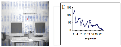
Fig. 5 – Evaluation of the VC.
3.3. Calculating the depth (intensity)
Using the optical flow field is calculated from two successive images, we can find information about the depth of each flow vector calculation by combining VC and speed of the robot while taking pictures.

where X – depth, V – is the speed of the robot, and T – VC (calculated for each optical flow vector).

Fig. 6 – Calculation of depth.
Fig. 6 shows an image depth, which is calculated by the VC. The darkest point is near, while the brightest point is the farthest from the scene, so the brightest point is the navigation area of ​​the robot.
3.4. Balance strategy for obstacle avoidance
The basic idea behind this strategy is offset (parallax) movement, the robot translates nearest objects rise to more rapid movement on the retina than more distant objects. He also takes advantage of the prospects that closer objects also occupy a larger field of view, rejecting the average with respect to the associative flow. The robot turns away from the stronger flow. This control law is formulated:

Here  the difference in the strength of the two sides of the body of the robot, and
  Is the sum of the magnitude of the optical flow in the visual field of the hemispheres on one side of the header robot.
We have implemented a strategy to balance our mobile robot. As we have shown in Fig. 7, the left optical beam (699, 24) is greater than the right (372, 03), so the solution is to turn to the right to avoid obstacles. (A chair to the left of the robot).

Fig. 7 – The result of the strategy of balance.
4. Experiments
The robot has been tested in our laboratory robotics, robot containing, office chairs, office furniture and computer equipment. In the next experiment, we test the ability of the robot to detect obstacles using only the strategy of balance.

Fig. 8 – Robot vision.
Fig. 8 shows a view from a camera robot initial snapshot.

Fig. 9 – The first decision.
Fig. 9 (a) shows the result of a strategy of balance in which robots have to turn right to avoid the nearest obstacle (the board), and Fig. 9 (b) shows the corresponding depth image, which is calculated from the vector of the optical flow. We see that the brightest point is localized to the right of the image, which determines the navigation area of ​​the robot.
Fig. 10 shows a robot when it turns to the right.

Fig. 10 – Robot vision.
Fig. 11 (a) shows the result of a balance strategy in which the robot must rotate to the left to avoid the walls, and Fig. 9 (b) shows the corresponding depth of the image in which the brightest point located on the left side of the image.
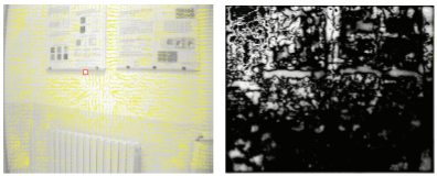
Fig. 11 – The second solution.


Fig. 12 – The robot is in motion.
Figure 12 (a) pokazyvet picture robot in motion in our laboratory, and Figure 12 (b) shows the path that passes by the movement of the robot. We notice that the robot found two principal positions, in which it changes the orientation, position (1) fit into the image and the position of the board (2) corresponds to the wall.

Fig. 13 – Schedule contact time.
Figure 13 shows a graph of left and right optical flow. At the beginning of the stream picture left more than the right, so the robot turns to the right, which corresponds to Figure 12 (d), then right flow increases until it is larger than the left, because the robot is approaching closer to the wall than to the board and we see an increase in the two columns (left and right flow) through the structure 13 in Figure 5, and then the robot turns left, to prevent the wall, it corresponds to position 2 in Fig. 12 (g). It can be seen that the robot successfully wandering around the lab, avoiding obstacles; however, we found that the lighting conditions critically important to detect obstacles, because the image produced by the camera is more noisy in low light and makes the optical flow estimation more wrong.
5. Conclusions
The article describes how the optical flow which provides the ability of the robot to avoid obstacles, use control laws, called “strategy of balance”, whose main purpose is to detect the presence of objects close to the robot on the basis of information on the movement of image brightness.
The main difficulty in the use of optic flow to navigate, is that it is unclear what is causing the change of gray values ​​(motion vector or changing the lighting).
Further improvement of the developed method is possible by connecting other sensors (sonar, infrared …), in cooperation with the sensor chamber.
6. Links
- Andrew, PD; William, H. & Lelise, PK (1998). Environmental Robotics. Adaptive behavior, Volume 6, No. 3/4, 1998
- Bergholm, F. & Argyros, A. (1999). The combination of central and peripheral vision to navigate reactive robot, in the basis of IEEE Computer Society Conference on Computer Vision and Pattern Recognition, Vol. 2, October 1999, pp. 356-362.
- Horn, KP & Schunck, BG (1981). Determining optical flow. Artificial intelligence, â„- 7, pp. 185-203, 1981.
- Negahdaripour, S. & Horn, KP (1989). The direct method is to place the focus of expansion, comp. Visible Graph. Strongly Protsess.46 (3), 303-326, 1989.
- Sandidni, G.; Santos-victor, J .; Curotto, F. & Gabribaldi, S. (1993). Divergent stereo navigation: learning in bees, in the proceedings of the Company IEEE Computer. Conference on Computer Vision and Pattern Recognition, June 1993, pp. 434-439.
- Santos-victor, J. & Bernardino, A. (1988). Visual behavior for binocular tracking, robotics and autonomous systems, with 137-148, 1998
- Tresilian, J. (1990). Perception information Timing of capturing action, Perception 19: 223-239, 1990
|
|
|
|
|
|
|


Cite This Work
To export a reference to this article please select a referencing stye below:
Related Services
View all


DMCA / Removal Request
If you are the original writer of this essay and no longer wish to have your work published on UKEssays.com then please click the following link to email our support team:
Request essay removal