Volumetric Glassware, Statistics, and Spreadsheet Exercise

Volumetric Glassware, Statistics, and Spreadsheet Exercise

Introduction

When one collects a set of data during an experimental procedure, statistical analysis is recommended in order to better understand what this data means. This lab aims to put different statistical and analytical methods to use on different types of data sets. Taking the mean of a set of data provides a typical representation for that set of numbers, and it may also provide the most probable future outcome, depending on the set of data. Taking the standard deviation of a set of data measures the spread of scores within that set. A low standard deviation signifies that most values are close to the average, while a high standard deviation signifies that the values are spread out. The relative standard deviation shows whether the standard deviation is small or large when compared to the mean and it also gives an idea on how precise the data is. A smaller relative standard deviation implies a more precise data set. In addition, a Gaussian distribution curve can be used to determine the frequency of occurrence of any value. Less precise results are indicated by a broader curve and a higher value of standard deviation. It isn’t out of the ordinary to obtain a value that’s much higher or much lower than any of the other values in the set; this value is called an outlier. In order to determine whether this value needs to be discarded, the Grubbs test must be utilized. However, the use of Grubbs test must be left as a last resort option. No method of statistical analysis can provide more accurate results than careful laboratory techniques. Overall, before resorting to using Grubbs test, the best option is to obtain more data points. Statistical analysis can also be used to determine the accuracy of a laboratory instrument, such as the true volume dispensed by a pipet.

 The main objective of this lab was the use of different statistical methods in order to determine the precision or accuracy of different data sets. In addition, volumetric operations were reviewed in order to prepare different dilutions whose concentrations needed to be calculated using the dilution equation and whose absorbance needed to be measured using a SpectroVis Plus. Also, this lab required the use of motorized pipets to calibrate the pipet. Additionally, this lab enforced the use of spreadsheets in order to analyze the data collected.

Experimental Section

A 03:50 dilution was prepared from the stock solution. Using a motorized pipettor, exactly 300 microliters of the stock solution were transferred into a 50 ml volumetric flask. The sample was diluted by adding distilled water to the flask until it reached the 50 ml mark. The molarity of this solution was calculated using the dilution equation. These steps were repeated to prepare a 0.5:50, 0.7:50, and a 0.9:50 dilutions, replacing the 300 microliters with 500 microliters, 700 microliters, and 900 microliters respectively. All dilutions were labeled as soon as they were prepared. Using a SpectroVis Plus, the absorbance of each of the 4 diluted standards was measured at the operational wavelength.

 A 5-ml pipette was obtained and cleaned. Some distilled water was obtained and its temperature was measured and recorded. A 25-ml Erlenmeyer flask was obtained and weighed while it was empty, this mass was recorded. Then, using the clean 5-ml pipette, 5 ml of distilled water were pipetted into the flask. The flask plus water was then weighed and this mass was recorded. At least 3 data points of the flask plus water were obtained, but the flask was not emptied and more water was not added. Subtraction was used to get the weight of the 5 ml of water added. This procedure was repeated, but replacing the 5-ml pipette with a 10-ml pipette, and the 25-ml Erlenmeyer flask with a 50-ml Erlenmeyer flask. The volume of water delivered was calculated using the equation: V_t=m_t/P_water, where P_water is the density of water.  Statistical analysis was used to determine the mean, standard deviation, and relative standard deviation for both the 5 ml and the 10 ml pipet. Use the equation: m_t=m_a+(V_waterP_air-V_weightsP_air) to calculate the true weight of water delivered (P_air is the density of air).

Results and Discussion

 The first section of the lab required the reading of volumes from a buret. The readings were done by different individuals and the buret was not touched during the readings, giving way to random error, which is a type of error than can’t be corrected regardless of the careful attention of the analyst. Statistical analysis was then used to determine the mean, standard deviation and relative standard deviation. Once the standard deviation was obtained, grubbs test was used to determine if there were any outliers, or points that deviated too far from the average and failed the grubbs test. Table 1 includes the volumes in ml collected from the buret readings, the deviation from the mean, and the deviation squared.

Table 1. Buret Readings

                    ∑=169.8                                     ∑=0.1000                                 ∑=9.418*10^-1

These values were then plotted to create a Gaussian curve, which depicts the frequency of occurrence of a value versus the value. Figure 1 depicts the Gaussian curve for the data set in Table 1, excluding the value 22.01 which was omitted using Grubbs test.

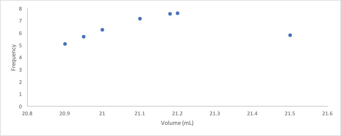
Figure 1. Gaussian curve of buret readings.

Mean: (21.18+21.10+20.90+21.00+21.50+21.20+20.95+22.01) / 8=

Mean=21.23 ml

Standard Deviation: √((9.418*10^-1)/(8-1))=

Standard Deviation=0.3668

Relative Standard Deviation: 0.3668/21.23=

Relative Standard Deviation= 0.01728 = 1.728% or 17.28 parts per thousand

Grubbs test: Gcalc= |22.01-21.23|/0.3668= 2.126. Gtable for (n=8)= 2.032

Grubbs test: Gcalc>Gtable = discard data point, 22.01.

From the data collected, only the precision of data can be analyzed. The readings were relatively close to the average, within a range of >0.34, except for the outlier value which deviated from the mean by 0.78. Grubbs test was used to determine that the volume 22.01 needed to be discarded since it deviated too much from the average. The accuracy and the percent error can’t be determined since there is no set value to compare the other readings too. One way to determine the accuracy would be to perform a calibration of the buret and calculate the true weights and volumes. The main source of error in this experiment was human error since all the readings were done by students. In addition, another error would be the mistake of some students to record a reading to 4 significant figures, which produced some readings with only 3 significant figures (a zero was added to these values), which takes away from the precision of results.

 Four diluted solutions were prepared from one stock solution whose concentration was calculated using its mass, 0.0808 g, and the volume of distilled water, 250.0 ml, as well as its percent purity, 91%. The concentrations of the diluted solutions were then calculated using the dilution equation. The absorbance’s of each of the diluted solutions was then measured using a SpectroVis Plus. The operational wavelength was 629 nm. Table 2 shows the concentrations (M) of the 4 diluted solutions as well as there absorbance’s (a.u).

Table 2. Molarity and Absorbance’s of Diluted Solutions

A calibration curve was then created using the calculated concentrations and the measured absorbance’s to show how absorbance, which is an experimentally measured property, depends on a known property, like the concentration of the standard. Figure 2 shows concentration (M) vs. absorbance (a.u.) for the data set in table 2. 

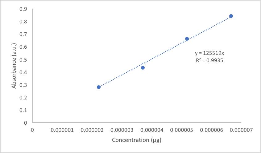
Figure 2. Absorbance as a function of concentration.

Concentration of stock solution: 0.0808g* 91% purity= 0.07353

0.07353g* (1mol/794.91g)= 9.250*10^-5 mol

9.250*10^-5/0.2500L= 3.700*10^-4 M

Concentration of 0.3:50 dilution: (3.700*10^-4))(0.3ml)=(M2)(50ml)

Concentration of 0.3:50 dilution: 2.22*10^-6 M

According to the calibration curve, the relationship between the absorbance and concentration is really dependent since the points lie on or not far from the line of linear regression. One method to determine the accuracy of these results is to use Beer’s law which depends on both concentration and absorbance. One source of possible error could lie in the preparation of the diluted solutions. It could either be human error with the addition of distilled water or it could be an error due to a faulty instrument. One visible observation was that as the volume of stock solution used increased, the intensity of the blue color of the solutions also increased. Overall, the statistical analysis using the calibration curve shows that the results were relatively accurate since they lied close to the line of linear regression.

 In order to determine the precision of volume dispensed by a pipet, the principle that water at a certain temperature has a given density and thus a given volume will have a certain mass was used. The mass of an empty flask was recorded along with the mass of the flask plus water. These values were then subtracted to get the mass of the water delivered into the flask. By using the equations for true weight and true volume, the true volume delivered by the pipet was calculated. The mean, standard deviation, and relative standard deviation were then calculated from these values. This was done with both a 5 ml and a 10 ml pipet. Table 3 shows the weight of flask, the weight of flask and water, the weight of water, the true weight of water, and the true volume of water.

Table 3.

Temperature of Distilled Water: 25ºC

True Weight for 5 ml pipet: m_t=m_a(((m_a/P_water)*P_air)-((m_a/P_steel)*P_air))

m_t= (4.9785)+((4.9785/1.000g/ml)*0.00110g/ml)-((4.9785/7.8002g/ml)*0.00110g/ml))

m_t= 4.98 g

True Volume for 5 ml pipet: V_t= m_t/P_water

V_t= 4.98g/1.000g/ml= 4.98 ml

Mean Volume for 5 ml pipet: (4.98+4.98+4.98)/3= 4.98 ml

Standard Deviation: √(((4.98-4.98)^2+(4.98-4.98)^2-(4.98-4.98)^2)/(3-1))= 0

Relative Standard Deviation: (0/4.98)*1000= 0

Percent error for 5 ml pipet: ((4.98-5ml)/5)*100= -0.4%

Percent error for 10 ml pipet: ((9.99-10)/10)*100= -0.1%

The three true weights and true volumes came out to be the same for each pipet respectively. This was mostly due to the rounding after the true weight calculation since the values only differed after the fourth significant figure. This lead to the standard deviation and relative standard deviation to come out to 0, since the values were all the same. However, this only indicates precision. Accuracy is determined by how far the true volume lies from the expected value, which is 5ml. By taking into affect different factors that might have an effect on the accuracy of measurements, one can achieve more accurate results, such as considering the buoyancy from air. Percent error is very low for both pipets, indicating a high level of accuracy for the pipets. However, more data points must be collected to further determine the pipettes accuracy.

Conclusions

This lab was successful in putting to use different methods of statistical analysis to determine the precision and/or accuracy of different data sets. Some of this data was then plotted. A Gaussian curve was used to analyze the frequency of different buret readings. Also, a calibration curve was used to depict the dependence of an experimentally measured property, absorbance, on a known value, concentration of standard. Grubbs test was used to determine whether a point should be kept or discarded, and it revealed that one point, 22.01, must be discarded from the data set in Table 1. The use of burets. flasks, and pipets further extended knowledge on volumetric operations and the dilution equation was used to determine the concentration of different dilutions. The calculated concentration of the stock solution was 3.700*10^-4 M while the concentrations for the 0.3:50, 0.5:50, 0.7:50, and 0.9:50 dilutions were 2.22*10^-6, 3.70*10^-6, 5.18*10^-6, and 6.66*10^-6 respectively. The percent error for the calibration of the 5 ml pipet was -0.4% while the percent error for the 10 ml pipet was -0.1%. The low percent error along with a standard deviation of 0 indicates precision and accuracy. But as for every experiment, more data points and more trials are needed to be able to solidify a conclusion that implies accuracy and precision.

References

• Instrumental Methods of Analysis Laboratory Manual, Department of Chemistry, Binghamton University, Binghamton, New York, 2011, pp. 39-49.