Use of Flourescent Plate Reader: Sampling of Heterogenous Solids

Abstract

A Gemini XPS microplate reader was used to determine if current mixing practices were able to produce uniform tablets capable of delivering a consistent quantity of the active ingredient, pyrenesulfonic acid (PSA).  Only the second dilution was picked to be analyzed since it contained the most consistent data with the lowest variance.  The variance of the second dilution tablet, ${\mathrm{\sigma }}_{\mathrm{tablet}}^2$

= 8.53621E-18 M², accounted for 8.037% of the total variance.  The average concentration of PSA for the second dilution among 9 PSA fluorescence readings was 4.430E-07 M ± 6.554E-09 M.  No outliers were present since no values fell outside of ±25% of the mean.  The total variance (σ_total²) was 1.06209E-16 M²; ${\mathrm{\sigma }}_{\mathrm{tablet}}^2$

was 8.53621E-18 M²; σ_measured² was  4.295E-17 M2; σ_preparation² was 5.47224E-17 M². Overall, the data analysis denotes significant variance in the concentration of PSA among the samples—proving that the current mixing process of solid sampling is inconsistent and in need of revision.  

Introduction

The purpose of this experiment was to test the homogeneity of tablet samples provided, and to determine the efficacy of solid sample mixing in delivering a consistent and precise amount of the active ingredient within a standard tablet.  PSA was used as the active ingredient due to its fluorescence quality, and Na₂SO₄ was used as an inactive suspension medium. The set-up for this experiment mimics the mixing process of pharmaceutical drugs.  Since the active ingredient is potent in microgram dosages, a seemingly small error would still deliver too much or too little of the active ingredient.  Delivering too much or too little of a high potency drug could cause unintended side effects or decreased efficacy—either case would mean endangering the life of the patient.

Fluorescence of PSA was measured using a Gemini XPS microplate reader, and samples were loaded onto a 96 well plate.  Standards prepared by the TA, a blank, and the replicates of three samples and their varying dilutions were loaded onto the well plate.  The fluorescence output from each cell is attained by bombarding the plate with photons.  The electrons of the fluorophore (PSA) is excited to a higher energy state by absorbing the photon of a shorter wavelength.  Energy is released, in this case light, as the PSA transitions from a higher energy state to a lower energy state.  The wavelength emitted is a longer wavelength.  This emission is picked up by the Gemini XPS reader and the intensity of the wavelength is reported.

The Gemini XPS reader utilizes light from an excitation source to emit photons at a sample.  The light is passed through a monochromator so that a specific wavelength can be selected–excitation wavelength is unique for each compound.  The sample would then absorb the photon and its valence electrons would then be excited to a higher energy state.  The electrons would then fall back to ground state, and in that process emit a wavelength.  A separate monochromator is used to separate the emission light from the excitation light.  And a photomultiplier tube is used to detect the fluorescence values.

Using the standards premade by the TAs, fluorescence values obtained from the Gemini XPS were used to plot a standard curve of fluorescence vs concentration of PSA in the standards.  A best-fit line can be obtained from the curve and concentration of the samples can be calculated using the best-fit line equation.  Data analysis was then carried out for the concentrations of the samples.

Experimental Methods

Materials:

• Mixture of 0.05 % w/w/ pyrenesulfonic acid and sodium sulfate
• 96 well plate
• Gemini XPS microplate reader
• Microliter pipet and tips (Eppendorf)
• Standard glassware
• Microfuge sample vials

Table of Physical Constants:

Procedure:

1. Standard solutions made by the T.A.

    10 total samples (9 standards + blank)

2. Transferred 100 µL of each standard onto well plate, starting with cell A1 and progressing downwards in columns
3. Weighed out three ~200 mg portions from pre-crushed tablet sample mixture—recorded weight

    Dissolvee each ~200 mg portion into individual 25 mL volumetric flask using DI water

    Transferred three -100 µL portions of each sample onto the 96 well plate (a total of 9 wells)—original concentration cells 

4. Successive dilutions:

    Took 100 µL of each sample at original concentration and placed into a separate microfuge vial

    Added 900 µL of DI water to each vial—agitated till combined

    Transferred 3 – 100µL portions of each diluted sample onto the 96 well plate

5. Repeated step 4 three more times to have four dilutions factors total.
6. Randomization of the cells was omitted since it was experimentally determined that variance between the wells is less significant than variance between samples.

    Because of this, samples were placed consecutively down the columns of the 96 well plate, starting a new column once last well was reached.

7. Gemini XPS plate reader was set to an excitation wavelength = 314 and an emission wavelength =  376. The 96 well plate was processed, and data is reflected in Table 1.
8. Data analysis was then ran on the recorded data

Results and Data Analysis

Fluorescence values of the standard solutions and one blank solution were used to construct a standard curve.  The concentration of pyrenesulfonic acid (PSA) vs fluorescence was plotted.  Standards highlighted in gold were used to construct the standard curve (Table 2).  At high concentration and at very low concentration Beer-Lambert Law is not applicable.  At high concentration solute-solute interactions dominate and a shift in absorption wavelength is observed.  Similarly, at very low concentrations solvent-solvent interactions dominate, also shifting the absorption wavelength.  Extreme lows and highs in concentration would result in a deviation from the linear curve, making the standard curve less accurate by decreasing the correlation of absorption and concentration.  Therefore, extreme highs and extreme lows in concentration were omitted to maximize the positive correlation between fluorescence and concentration of PSA.

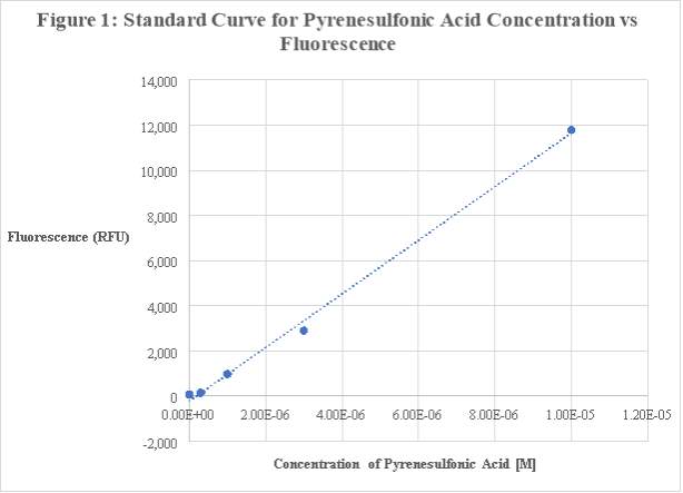
*Note: The best-fit line does not intersect the origin because the fluorescence of the blank was not zero—due to scattered light.

R² = 0.9969 denotes a strong positive correlation between fluorescence and concentration of PSA.

The best-fit line equation was determined to be: y = (1.19 E9)x – 217.82               (eq. 1)

Concentration of PSA was determined by using the best-fit line equation wherein average fluorescence value was used as the y input.  Concentration can then be calculated by solving for x.  The concentration of each sample was determined, and the concentration of the individual dilutions were also calculated in a similar fashion.

e.g.  Avg Fluorescence = (1.19 E9)*[PSA] – 217.82      (eq. 2)

Histogram

A histogram was not performed since there were only 3 samples measured.  The lab procedure was altered so that four dilutions were made from each sample.  Because the data obtained was not that of a single homogenous population, a histogram would be misleading to identify subpopulations as the varying levels of dilution factors themselves can be considered subpopulations. 

Standard Deviation of Population

An overall average was taken of the average concentrations provided in Table 3.  Original concentrations of all samples were averaged to obtain the overall average concentration; the same procedure was followed for the subsequent dilutions.

Standard deviation was calculated using:  STDEV = $\sqrt{\frac{\sum _{\mathrm{i}=1}^{\mathrm{n}}{({\mathrm{x}}_{\mathrm{i}}–\bar{\mathrm{x}})}^2}{\mathrm{n}–1}}$

                 (eq 3)

Coefficient of Variation (CV) at each various concentration was calculated using:

Coefficient of Variation (CV) = (STDEV/ Average) x 100          (eq 4)

The coefficient of variation of the second dilution was lowest—denoting that dilution 2 had the least amount of variation relative to its mean.  Since dilution two had the least amount of variability, it was instructed that an ANOVA should be ran for only the second dilution.

To identify any outliers, it was decided to isolate concentrations that is greater than +/- 25% from the mean.  The procedure is the same for the original concentration and all the subsequent dilutions.  Calculations for the original concentration will be used as an example.

Upper Boundary of [Original] = Mean + (.25)(Mean)       (eq 5)

Upper Boundary of [Original] = 1.976E-05 + (.25)( 1.976E-05) = 2.470E-05 M

**No concentration values fell above the upper boundary for the [Original] concentration data pool.

Lower Boundary of [Original] = Mean – (.25)(Mean)       (eq 6)

Lower Boundary of [Original] = 1.976E-05 – (.25)( 1.976E-05) = 1.482E-05 M

**No concentration values fell below the lower boundary for the [Original] concentration data pool.

It was determined that there were no outliers within the data.  Refer to Table # in appendix for the lower and upper bounds of each dilution.

ANOVA

An ANOVA: Single Factor Analysis was performed to determine the level of variance between the tablet samples.  It was instructed that ANOVA would be run for the second dilution only since the concentration fits within the standard curve; the second dilution also has the lowest coefficient of variation (i.e. 1.479% error)(Table 4).

The concentrations of all the replicates of the second dilution were calculated using the line of best-fit equation (eq 1); the data is shown in Table 3.  Using the average concentrations, Table 5 represents the sum, average, and variance of each sample’s second dilution.

Table 6 is a summary of the ANOVA output.  MS_within represents an estimate of the variance in measurement technique, σ².  MS_between represents σ²+n σ_tablet², where n is the number of replicates and σ_tablet² is the variance due to the differences among the tablet samples (1).

**Note: SS = Sum of Square, df = Degree of Freedom, MS = Mean Square, F = F_calculated

Since F_calculated < F_critical and P-Value(0.612762098) > α(0.05), there is significant probability that the variance between groups were due to random data fluctuations—on a 95% confidence interval.

The total variance can be calculated by (2): 

σ_total² = σ_tablet² + σ_preparation² + σ_measured²                         (eq 7) (2)

σ_preparation²

σ_preparation² = MS_within                  (eq 8) (1)

σ_preparation² = 5.47224E-17 M²

σ_measured²

σ_measured² = (6.554E-09M)² = 4.295E-17 M²                          (eq 9) (1)

*using standard of deviation value from Table 4

σ_tablet²

${\mathrm{\sigma }}_{\mathrm{tablet}}^2=\left|\frac{{\mathrm{MS}}_{\mathrm{between}}–{\mathrm{MS}}_{\mathrm{within}}}{\mathrm{n}}\right|$

              (eq 10) (1)

${\mathrm{\sigma }}_{\mathrm{tablet}}^2=\left|\frac{(2.91138\mathrm{E}–17)–(5.47224\mathrm{E}–17)\mathrm{ }}{3}\right|$

${\mathrm{\sigma }}_{\mathrm{tablet}}^2=\mathrm{ }$

8.53621E-18 M²

σ_total²

σ_total² = 8.53621E-18 M² + 5.47224E-17 M² + 4.295E-17 M²            (eq 7) (2)

σ_total² = 1.06209E-16 M²

Therefore, %variance due to tablet variance = $\frac{{\mathrm{\sigma }}_{\mathrm{tablet}}^2}{{\mathrm{\sigma }}^2\mathrm{total}}$

x 100 = 8.037181406 %.                      (eq 11)

Discussion

The purpose of this experiment was to test if each tablet sample consistently delivered the same amount of the active ingredient in a drug.  PSA, a fluorophore, was used to represent the active ingredient in a drug.  A Gemini XPS reader was used to detect the fluorescence of PSA in each sample.  Concentration was then calculated using the best-fit equation of the standard curve, y=(1.19 E9)x – 217.82, wherein the standards of PSA was plotted against their fluorescence output.  An R² = 0.9969 confirms a positive correlation between the standard’s PSA concentration and its fluorescence output.  It is important that the concentration of Na₂SO₄ is equivalent in the standard and the sample tablets so as to not introduce errors in the fluorescent output.  Additionally, deionized water should be used to make the solutions so that there is not additional errors via ion-ion interactions.

Five separate concentrations were made of PSA; the first being the original concentration, and then four subsequent dilutions of each sample diluted by a factor of 10.  The various concentrations of each sample was labeled original, 1^st dilution, 2^nd dilution, 3^rd dilution, 4^th dilution.  After computing the coefficient of variation (CV) for the overall average of all the samples (i.e. CV was calculated from average original concentration of all the samples, same procedure for subsequent dilutions), dilution 4 was omitted.  The coefficient of variation (CV) for most of the concentrations were similar, with the exception of the 4^th dilution—which was too dilute to yield good data so was therefore omitted.  More importantly, since the CV of the second dilution was close to that of the original concentration, analyzing the variance of the second dilution would yield good correlation on the whether or not the homogeneity of the tablets are consistent at their original concentration.

Only the second dilution was picked to be analyzed since it contained the most consistent data with the lowest variance.  The average concentration of PSA for the second dilution among 9 PSA fluorescence readings was 4.430E-07 M ± 6.554E-09 M.  No outliers were present since no values fell outside of ±25% of the mean.  The total variance (σ_total²) was 1.06209E-16 M²; ${\mathrm{\sigma }}_{\mathrm{tablet}}^2$

= 8.53621E-18 M²; σ_measured² = 4.295E-17 M2; σ_preparation² = 5.47224E-17 M²; and 8.037% of the total variance was from variance within the tablet samples.  Overall, the data analysis denotes significant variance in the concentration of PSA for the second dilution.  Considering that the second dilution had the lowest variance out of all the dilutions and the original concentration, it stands that variance is even worse for the original concentration and the other dilutions.

ANOVA was ran and a p-value of 0.613, with an F_calculated of 0.532026526 and an F_critical of 5.14325285 . Since P-Value(0.612762098) > α(0.05), there is significant probability that the variance between groups were due to random data fluctuations (on a 95% confidence interval).

It is clear from the data that non-homogeneity is an issue.  Variations of the tablets can be from ineffective mixing and/or imprecise sampling.  Since the drug is high potency, variation in a milligram tablet would cause a significant variation when the active ingredient is on a microgram scale.  Delivering too much or too little of a high potency drug would mean endangering the life of the patient.  A way to troubleshoot this issue is to individually compound the tablets and have the process automated.  In this case, an exact dose of the active ingredient is added to an exact amount of carrier compound.  Cost and time, however, would be mitigating factors since tablets are compounded individually.

References

1. CHEM 3472-002 Lab reading, “Use of Fluorescent Plate Reader/ Sampling of Heterogenous Solids”
2. Guy, Robert D., et al. “An Experiment in the Sampling of Solids for Chemical Analysis.” ACS Publications, pubs.acs.org/doi/abs/10.1021/ed075p1028
3. “Microplate Reader: Plate Reader – BMG LABTECH.” BMGLabtech.com, www.bmglabtech.com/microplate-reader/.
4. Newton, et al. “Ultraviolet-Visible (UV-Vis) Spectroscopy – Limitations and Deviations of Beer-Lambert’s Law: Analytical Chemistry.” PharmaXChange.info, 27 June 2016, pharmaxchange.info/2012/05/ultraviolet-visible-uv-vis-spectroscopy-%E2%80%93-limitations-and-deviations-of-beer-lambert-law/.

Appendix