Budget variance analysis guide

Stuck on budgeting complexities or tough variance analysis? Let our qualified accountants handle your assignment – accurate, reliable, and stress-free. Visit our accounting assignment help page for info.

Budgeting is a fundamental part of managerial planning and control. It provides a system of planning, coordination and control for management (ACCA, n.d.).

Managers use budgets to set financial targets and allocate resources for a period. They then compare actual performance against these plans.

Variance analysis is the process of comparing actual results with the budgeted figures and analysing the differences. It helps managers understand why results differ from expectations and to take corrective action if needed (Clarke, 2025). For example, if actual costs exceed the budget, variance analysis pinpoints which costs are higher and why.

Variances are commonly labeled as favourable (better than expected) or adverse (worse than expected) (Clarke, 2025). Managers typically focus on significant variances – those that are large or unusual. These variances highlight areas that may require attention (CFI Team, n.d.). This guide first explains the key types of budgets (incremental, zero-based and flexible). It then outlines how to calculate major variances (sales, materials, labour and overheads). Finally, it provides advice on interpreting variances and linking the numbers to managerial decisions.

Types of budgets

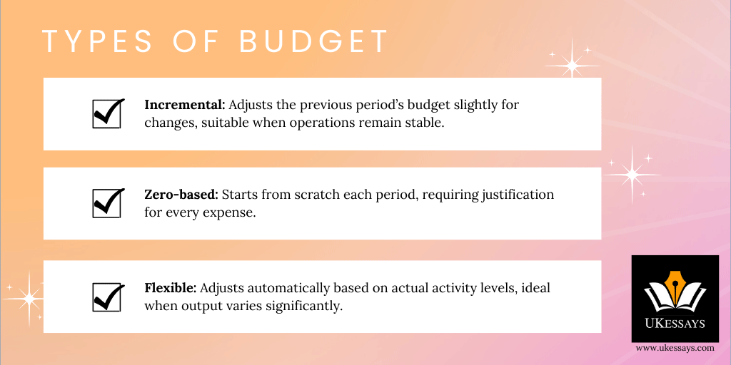
Organisations can prepare budgets using different methods, each with advantages and drawbacks. The choice of budgeting approach affects how the budget is constructed and how much scrutiny is applied. Three common budgeting methods are incremental budgeting, zero-based budgeting and flexible budgeting.

Incremental budgeting

Incremental budgeting is a traditional method where last period’s budget (or actual results) is used as the base for the new budget, with incremental adjustments added for the upcoming period (ACCA, n.d.). These adjustments might include factors like inflation or planned growth in sales and costs.

The approach is simple and quick, making it easy for managers to implement and understand. It requires relatively little analysis of each line item – the budgeter simply takes last year’s figures and increases them slightly (often by a set percentage) for the next year. This simplicity can save time and reduce conflict in the budgeting process (ACCA, n.d.).

However, a major drawback is that incremental budgeting tends to perpetuate existing inefficiencies (ACCA, n.d.). Managers are not forced to justify the baseline expenses, so wasteful or unnecessary costs can continue year after year.

There is little incentive to cut costs or innovate. Departments often assume they will get a similar budget as before (plus a bit more) regardless of actual need. Thus, incremental budgeting provides stability, but it can also lead to budgetary slack and inertia in the organisation’s cost structure.

Zero-based budgeting

Zero-based budgeting (ZBB) is a more rigorous approach that starts every budget line at zero. Managers must justify every expense for each new period (ACCA, n.d.).

Instead of assuming last year’s level of spending is automatically needed again, each department builds its budget from scratch based on its functions and plans. Managers prepare detailed “decision packages” explaining each activity’s purpose, cost and alternatives, to secure funding approval.

This method aims to allocate resources optimally to where they are most needed. This is because expenditures with insufficient justification do not receive funding (ACCA, n.d.).

The benefits of ZBB are substantial. They include eliminating outdated or inefficient activities and encouraging a critical, questioning attitude among managers towards all spending (ACCA, n.d.). By not simply carrying over last year’s figures, ZBB can curb wasteful spending and ensure each dollar or pound has a purpose.

On the downside, zero-based budgeting is very time-consuming and costly to implement. Preparing and reviewing the detailed packages requires significant effort and managerial skill. In a large organisation, doing ZBB for every department every year can be impractical. This is due to the sheer amount of analysis and documentation involved.

For this reason, some companies use ZBB selectively (e.g., every few years or for certain high-cost areas). They do this rather than implementing ZBB annually for all budgets.

When used wisely, ZBB can lead to a more efficient allocation of resources, but its complexity means it needs strong management support.

Flexible budgeting

A flexible budget is a budget that adjusts to the actual level of activity (such as actual sales volume or production volume) rather than remaining fixed at one level.

A static budget (fixed budget) is set for only one level of output and does not change. By contrast, a flexible budget is recalculated based on the actual outcomes. It essentially provides a budgeted cost and revenue figure for the actual activity achieved.

For example, if a company budgeted costs for making 10,000 units but actually produces 12,000 units, a flexible budget would increase the allowed expenses in proportion to the higher volume. This creates a more realistic benchmark for comparing actual costs.

Why choose a flexible budget:

A flexible budget is particularly useful in variance analysis and performance evaluation because it separates volume effects from other factors. Using the same actual activity level for both budget and actual makes the reported variances more meaningful (Bragg, 2024).

In fact, variances computed with a flexible budget tend to be smaller and more relevant, since they highlight differences due to efficiency or price changes rather than simply output volume differences (Bragg, 2024).

Preparing a flexible budget requires identifying which costs are fixed and which are variable, and understanding how variable costs change with activity. Fixed costs remain the same in the flexible budget, while variable costs are adjusted according to the actual volume.

Overall, flexible budgeting adds sophistication to the budgeting process by acknowledging that business activity can deviate from the forecast. It provides management with a “what if” tool to evaluate financial performance at different levels of activity.

In practice, a company may prepare budgets for multiple scenarios or use formula-based models to compute expected costs and revenues for the actual output. The flexible budget approach enhances control by ensuring that managers are evaluated against a budget that matches the actual operating conditions. This practice makes performance appraisal fairer and more accurate.

Variance analysis in management accounting

After the budget period concludes, managers compare the actual results to the budgeted figures and investigate the differences. This process is known as variance analysis. Put simply, a variance is the difference between the expected outcome (budget or standard) and the actual outcome achieved.

Variance analysis provides a quantitative lens to assess where the organisation over-performed or under-performed (CFI Team, n.d.). The sum of all variances gives an overall sense of performance. It indicates whether the company beat its budget or fell short in that period.

More importantly, examining individual variances (for specific revenue or cost items) helps identify problem areas or successes. For each significant variance, managers will ask:

• Cause – What likely caused this variance?
• Impact – Why does it matter?
• Action – What should we do about it, or what decisions does this inform?

By answering these questions, managers can turn the variance numbers into actionable insights.

Classification: favourable or adverse variances

It is crucial to classify variances as favourable (F) or adverse (A).

• A favourable variance means the actual result improved profit relative to budget (for example, higher revenue or lower costs than planned).

• An adverse variance means profit was worse than budget (for instance, lower sales or higher costs than expected).

For example, spending £50,000 less than budgeted on materials would be a £50,000 favourable variance (because it saves money). However, selling £50,000 less than expected in revenue would be £50,000 adverse.

Labelling variances in this way helps direct management’s attention. Typically, large adverse variances are of greatest concern. However, large favourable variances also warrant explanation – perhaps targets were too easy or luck played a role.

When conducting variance analysis, one important technique is using a flexible budget to isolate the impact of volume changes. Managers adjust the original budget to the actual sales or production volume before comparing with actual results. This ensures that differences caused solely by changes in output volume are removed.

By flexing the budget, the remaining variances show pure price or efficiency differences. This makes the analysis fair. Managers are not “penalised” for selling fewer units if those units simply could not be sold. The sales volume effect is reported separately. Using a flexible budget thus yields variances that are more actionable (Bragg, 2024).

Variance analysis typically focuses on a few key areas: sales, materials, labour and overheads. We examine each of these categories below, including how to calculate the variances.

Sales variances

Sales variances explain why actual sales revenue differed from the budget. There are two main components: the sales price variance and the sales volume variance. The sales price variance measures the effect of selling at a different price than planned. The formula is:

Sales Price Variance = (Actual Price – Budgeted Price) × Actual Quantity sold

If the actual selling price is lower than the budgeted price, the variance is adverse (because revenue was lower per unit than expected). If the actual price is higher, the variance is favourable (more revenue per unit). The sales volume variance measures the effect of selling a different quantity than planned. One way to compute it in revenue terms is:

Sales Volume Variance = (Actual Quantity – Budgeted Quantity) × Budgeted Price

This shows how the change in sales volume impacted revenue, holding price constant at the budgeted level. (In some cases, especially in profit analysis, sales volume variance is calculated using the budgeted profit or contribution per unit to show the impact on profit rather than revenue. But the concept is similar – it isolates the volume effect.)

Example:

Suppose a company budgeted to sell 1,000 units at a price of £10 each, for £10,000 of revenue.

In reality, it sold 1,200 units at an average price of £9 each, for £10,800 actual revenue.

The sales price variance = (£9 – £10) × 1,200 = £1,200 adverse.

This reflects that a £1 price cut on 1,200 units caused £1,200 less revenue than if the price had been £10.

Meanwhile, the sales volume variance = (1,200 – 1,000) × £10 = £2,000 favourable.

Selling 200 extra units (20% more volume) generated £2,000 more revenue than the original budget.

Together, the net sales variance is £800 favourable (£2,000 F – £1,200 A).

This means actual sales revenue was £800 above budget overall.

In this case, a manager’s analysis would note that the company gave a discount (leading to an adverse price variance, perhaps due to competitive pressure or a promotion). However, higher demand offset this by volume (a favourable variance).

Sales variances help managers understand whether revenue shortfalls or gains arose from price factors (like discounts, market pricing or product mix) or volume factors (like demand fluctuations or sales effort). This insight allows managers to respond accordingly in pricing strategy or marketing.

Material cost variances

Material variances examine the cost of raw materials used in production. They are usually split into material price variance and material usage (quantity) variance. The material price variance reflects paying a different price per unit of material than expected. The formula is:

Material Price Variance (MPV) = (Actual Price per unit – Standard Price per unit) × Actual Quantity of material used

“Standard price” is the budgeted (or standard) cost per unit of material (set in advance). If the actual price paid to suppliers is higher, the variance is adverse (since spending was more than planned for the materials actually purchased or used). If the actual price is lower, the variance is favourable.

The material usage variance (also called material quantity variance) reflects using a different amount of material than the standard allowed for the actual output. The formula is:

Material Usage Variance (MUV) = (Actual Quantity of material used – Standard Quantity allowed for output) × Standard Price per unit

The “standard quantity allowed” is the material input that should have been used for the actual level of production, according to the budget or engineering standard.

If actual material usage exceeds the standard allowance (perhaps due to wastage or inefficiency), the variance is adverse. Using less material than expected (through efficiency or less waste) would be favourable.

Example:

A company budgets that producing 1,000 units should require 2 kg of material per unit, at a standard price of £5 per kg. So the material cost budget is £10,000 (2,000 kg × £5).

Now say the company actually produced 1,000 units, but in doing so it used 2,100 kg of material, and the actual price paid was £5.20 per kg.

Actual material cost = 2,100 kg × £5.20 = £10,920.

We calculate the variances:

• Material Price Variance: Compare actual price (£5.20) to standard (£5.00) on the actual quantity used (2,100 kg). MPV = (5.20 – 5.00) × 2,100 = £0.20 × 2,100 = £420 adverse. Materials were £0.20 per kg more expensive than planned, costing an extra £420. The purchasing manager might note that suppliers raised prices or perhaps the purchasing team opted for a higher-grade material.
• Material Usage Variance: Compare actual quantity used to standard quantity allowed for the output, at the standard price. MUV = (2,100 kg – 2,000 kg) × £5.00 = 100 kg × £5 = £500 adverse. The company used 100 kg more material than expected for the volume produced, costing £500 more. This could be due to inefficiencies or waste in production (e.g., higher scrap rates).
• Total Material Cost Variance: £420 A + £500 A = £920 adverse. Actual material cost (£10,920) exceeded the budgeted cost for that output (£10,000) by £920.

In this example, the material price variance and usage variance together explain why material costs were over budget.

Management would investigate both aspects: Why did the price increase (supplier issues or market price changes?) and why was material usage higher (production waste, scrap or quality issues?).

By analysing material variances separately, companies can take targeted actions. For example, they might negotiate bulk discounts or improve quality control to reduce waste. This provides more insight than simply noting that materials were over budget.

Labour cost variances

Labour variances (for direct labour) are analogous to material variances. They reveal whether a company paid more or less for labour than expected, and whether labour was used efficiently.

The two components are labour rate variance and labour efficiency variance.

The labour rate variance (LRV) measures the difference between the actual wage rate paid and the standard (budgeted) wage rate for the actual hours worked. If the company paid a higher actual wage rate than the standard (e.g., due to overtime premiums or wage increases), this variance is adverse. It raises costs. Paying below the standard rate (perhaps by using lower-paid or less experienced staff) would yield a favourable variance.

The labour efficiency variance (LEV) measures productivity: it compares the actual hours taken to produce the output to the standard hours that should have been taken. The formula is:

Labour Efficiency Variance = (Actual hours worked – Standard hours allowed for actual output) × Standard hourly wage

If workers take more time than expected to complete the work, the variance is adverse (because extra labour hours were needed). If they work more quickly and use fewer hours, the variance is favourable.

The standard hours allowed refers to the labour hours that should have been used for the actual production, based on the standard labour time per unit.

Interpreting Labour Variances:

An adverse labour rate variance might occur if there was unplanned overtime (which pays a higher rate) or a wage rate increase that the budget did not factor in. This tells management that labour cost per hour was higher than expected.

Possible responses could be to review overtime policies or update the wage standards.

An adverse labour efficiency variance indicates lower productivity – workers took more hours than they “should” have for the output. Possible reasons include inadequate training, worker fatigue or machine breakdowns causing delays.

In contrast, a favourable efficiency variance means time saved. This could result from a learning curve, better training, improved processes or using more skilled labour than planned.

Just like with materials, separating the rate and efficiency effects helps managers target their actions. For example, they can address wage issues or productivity issues specifically.

Labour variances, material variances and variable overhead variances all follow the same pattern. Each has a price (rate) variance and a usage (efficiency) variance (CFI Team, n.d.).

Overhead variances

Overhead refers to indirect costs, which can be variable overhead (costs that vary with output, such as electricity for machines, indirect materials or machine maintenance supplies) or fixed overhead (costs that remain fixed in total, such as factory rent, supervisor salaries or depreciation).

In standard costing and variance analysis, overhead variances are typically examined in these categories:

Variable overhead variances:

These are often analysed similarly to labour variances because variable overhead is usually applied based on labour hours or machine hours.

We consider a variable overhead spending variance and a variable overhead efficiency variance.

The spending variance is like a price variance: it measures whether the actual cost per machine-hour or labour-hour of overhead was higher or lower than the standard rate.

The efficiency variance looks at whether the usage of the allocation base (machine hours, labour hours, etc.) was efficient relative to the standard.

• For example, if production takes more machine hours than expected, variable overhead costs (like power or supplies) increase. This yields an adverse efficiency variance.
• For example, a variable overhead spending variance could occur if electricity rates increased unexpectedly.
• Similarly, an efficiency variance might occur if machines had to run longer due to production inefficiencies.

Fixed overhead variances:

Fixed costs are budgeted in total, not per unit. Variance analysis separates the fixed overhead budget variance and the fixed overhead volume variance.

The fixed overhead budget variance (or spending variance) is the difference between actual fixed overhead incurred and the budgeted fixed overhead for the period.

Since fixed costs ideally remain unchanged with volume, any difference here may be due to cost control issues (e.g., an unplanned repair or higher utility expense).

The fixed overhead volume variance indicates how fixed cost per unit changes when actual output differs from the budget. It essentially shows the under- or over-absorption of fixed overhead. The formula often given is:

Fixed Overhead Volume Variance = Budgeted fixed overhead – Fixed overhead absorbed to actual output

If a company produced fewer units (or hours) than planned, then less of the fixed overhead is absorbed. The result is an adverse volume variance, because the business paid for capacity it didn’t fully utilise.

Conversely, producing more than planned absorbs more fixed overhead. This gives a favourable volume variance, as the fixed cost per unit is lower than expected.

For example, if a factory budgeted £100,000 of fixed overhead for a certain output but actual output was lower, there would be an adverse volume variance due to under-utilised capacity.

On the other hand, if output was 11,000 units (above the 10,000 planned), the volume variance would be favourable. The fixed cost per unit would be lower than expected.

Fixed overhead volume variance is important for understanding utilisation of resources (like plant capacity).

Summing up overhead variances:

To sum all this up, overhead variances indicate how well managers controlled indirect costs and how fully the firm utilised its capacity:

• An adverse variable overhead spending variance might prompt management to investigate increases in indirect material prices or waste of supplies.
• An adverse fixed overhead budget variance could trigger a review of fixed expenditures to find any overspending.
• A significant fixed overhead volume variance (adverse) would make managers evaluate why production volume fell short (e.g., insufficient demand or production bottlenecks). They might decide to adjust the production plan or marketing effort to improve utilisation of capacity. Management could also review whether any fixed costs can be reduced or deferred if demand remains lower.

These insights guide decisions on cost control and operational planning.

Interpreting variances and taking action

Calculating variances is only the first step – the ultimate goal of variance analysis is to understand why the variances occurred and what managerial actions should follow.

In financial reports, a list of variances without explanation has limited value. Managers need to provide a commentary that links the numbers to business realities. Writing an effective variance analysis commentary involves explaining the causes of variances and discussing their implications and potential responses.

A useful approach is to consider each significant variance and address the cause, impact and action as noted earlier.

For example, an adverse material usage variance might be explained by noting,

“We used 100 kg more material than standard, possibly due to higher scrap and waste.

Impact: This increased material cost by £500 and indicates an efficiency problem.

Action: We will investigate the production process for causes of waste.

We should also improve quality control and operator training to prevent this.”

In this way, the commentary identifies the root cause and suggests a remedy.

Another example: consider an adverse labour rate variance. A possible commentary could be,

“Labour costs were £X above budget because we had to pay overtime at premium rates (adverse rate variance).

Impact: This increased our payroll costs and reduced profit.

Action: Going forward, management will consider better production scheduling and hiring additional staff in peak periods. The aim is to reduce overtime.”

If there was a favourable labour efficiency variance, the commentary might say,

“We achieved a favourable labour efficiency variance of £Y, as the production team completed the work in fewer hours than anticipated.

Impact: This saved labour costs and suggests higher productivity.

Action: This positive outcome (possibly due to the new training program) is one we will seek to maintain and build on.”

In writing variance commentaries, the tone should be analytical and proactive. Rather than just stating “Variance X is adverse due to Y,” effective commentary will add interpretation and response: for instance, “…therefore we will do Z.” The goal is to connect the numbers to managerial decisions such as cost control measures, process improvements or strategy adjustments.

It’s also important to note whether variances indicate issues with the budgeting process itself. For example, consistently large favourable variances might mean managers set budgets too conservatively (making targets too easy). Conversely, large adverse variances might suggest the budget was unrealistic or that there were unforeseen external changes. Managers can use this feedback to improve future budgets or standards (Russell, 2024).

Finally, effective variance analysis and commentary closes the loop in the management control cycle: managers set plans (budgets), measure actual results against the plan (yielding variances), and then take actions to correct course or capitalise on successes. This continuous improvement cycle is at the heart of management accounting.

Identifying and explaining variances is essential since they “hold the keys to better future performance” (Russell, 2024). By deeply understanding the story behind the numbers, managers can make informed decisions to tighten cost control, adjust strategies and improve the organisation’s overall performance.

Stuck on budgeting complexities or tough variance analysis? Let our qualified accountants handle your assignment – accurate, reliable, and stress-free. Visit our accounting assignment help page for info.

References and further reading:

• ACCA (n.d.). Comparing budgeting techniques (Incremental v ZBB). [Online]. Available at: https://www.accaglobal.com/ (Accessed 9 September 2025).
• Bragg, S. (2024). Flexible budget definition. AccountingTools. [Online]. Available at: https://www.accountingtools.com/articles/flexible-budget (Accessed 9 September 2025).
• Clarke, R. (2025). Variance Analysis: A Simplified Explanation. aCOWtancy Blog, 1 Mar 2025. [Online]. Available at: https://www.acowtancy.com/blog/variance-analysis-in-5-mins (Accessed 9 September 2025).
• CFI Team (n.d.). Variance Analysis. Corporate Finance Institute. [Online]. Available at: https://corporatefinanceinstitute.com/resources/accounting/variance-analysis/ (Accessed 9 September 2025).
• Russell, B. (2024). Variance reporting: What is it + how to read/write a variance report. Cube Software Blog, 22 Mar 2024. [Online]. Available at: https://www.cubesoftware.com/blog/variance-reporting (Accessed 9 September 2025).