A Review of Magnetic Resonance Imaging

Computational MRI project- A Review of Magnetic Resonance Imaging

1. The anatomy

Simplistically, the process of obtaining an MR image entails the patient being placed on a magnet, application of a radio wave, radio wave being turned off, signal emission by patient, reconstruction of the image.

MRI scanners are composed of a magnet, shims, radio frequency apparatus, gradient coils, patient table and computer system.

The magnet is arguably the most crucial component; the magnetic field is produced by current flow through multiple coils within the magnet- this creates a state of superconductivity which reduces the resistance in the wiring to null values and induces the field.

Get Help With Your Essay

If you need assistance with writing your essay, our professional essay writing service is here to help!
Find out more about our Essay Writing Service

Magnetic field strength is measured in either tesla or gauss, with routine clinical scanners creating a field of 0.2 to 3.0 tesla; the Human Connectome Project has utilized fields ranging from 3.0 to 7.0T; some research facilities can produce fields of 11.7T and there is work underway to build a 20T field. (1)(2). It is expected that magnetic fields above 14 T will allow in vivo imaging at resolutions of less than 100 μm, while maintaining compatibility with health and safety limits. (2)

Augmenting the magnetic field yields better spatial and spectral resolution for medical imaging- it increases the signal-to-noise ratio. However, increases in magnetic field strength have been described to provoke side effects in humans, such as nystagmus, vertigo and peripheral nerve stimulation due to Lorenz forces (2) However, these health effects have been deemed to be innocuous and reversible in fields up to 9.4 T. Rodent studies have showed the same array of effects is observed and reversible in fields up to 21T. Research of safety limits is underway for humans (2).

Shims reduce inhomogeneities in the field; magnetic field homogeneity refers to the uniformity of a magnetic field in the centre of a scanner when no patient is present and is measured in parts per million (ppm). Shims can be either coils or steel, which respectively produce active shimming or passive shimming. In either case, both create additional magnetic fields that add to the external magnetic field as to increase the homogeneity of the field.

The second component is the radio frequency apparatus; the radio frequency (RF) transmission system consists of an RF synthesizer, power amplifier and transmitting coil and the receiver system consists of the coil, pre-amplifier and signal processing system. The interaction of an RF pulse with the tissues to be image will be discussed in detail later in this essay.

With regards to gradient coils, three gradient coils are located within the main magnet, producing three different magnetic fields that are weaker than the main field. Gradient coils are used to selectively superimpose the main field and spatially encode the positions of protons by varying the total magnetic field linearly across the imaging volume. The Larmor frequency will then vary as a function of position in the x, y and z-axes.

The patient table simply carries the subject of study into the bore. Patient position is determined by the part of the body that is to be scanned. Once the region of interest is in the isocentre- the exact centre of the magnetic field- the scanning process is started.

Lastly, the computer system, powerful technology that has the easy job of reconstructing the signal onto images that serve researchers and clinicians alike.

1. Electromagnetism

MRI technology is based on the property of nuclear magnetic resonance (NMR). The fulcrum of this revolutionary technology is the proton.

Proton in the context of NMR refers to hydrogen-1 nuclei in organic molecules. This method uses the spin of the proton, a form of angular momentum, which has the value one-half. In simple terms, as the proton’s positive charge moves around, it induces an electrical current, which in turn produces a magnetic field.

When the external magnetic field B0 is applied, spins can assume two positions, parallel or antiparallel with B0. These two alignments are on different energy levels. The lowest energy level is parallel alignment, and hence the preferred one. The difference in number of protons occupying either distribution is small and depends on the strength of the applied magnetic field. This can be quantified by spin excess as defined by

$\mathit{spin\; excess}=N\frac{h^{–}w0}{2\mathit{kT}}$

Where k is the Boltzmann constant and h ̄ω0, is the Larmor precession frequency where h ̄ ≡ h/(2π) with Planck’s quantum constant h.

For about 10 million protons in parallel alignment there are about 10 000 007 in the higher energy state.

When B0 is applied, the spins precess around field lines, and the precession frequency is proportional to the strength of the magnetic field. It can be calculated by the Larmor equation:

$w0=\mathit{gammaB}0$

Where w0 is the precession frequency (in Hz or MHz), B0 is the external magnetic field strength in Tesla and gamma is the gyro-magnetic ratio; this is 42.5 MHz/T for protons.

Parallel and antiparallel spins cancel each other out. However, as mentioned there is a small surplus of spins in the lower energy state. This creates a magnetic vector in the direction of the external magnetic field (z-axis by convention), which is denominated longitudinal magnetization.

As previously mentioned protons have spin which implies intrinsic angular momentum; in the knowledge that the external magnetic field exerts a displacement, a twisting or torque on the magnetic moment of the protons, we obtain the fundamental equation of motion.

$\frac{d\stackrel{⃑}{u} }{\mathit{dt }}=\mathrm{\gamma } \stackrel{⃑}{u} \stackrel{⃑}{B}$

3. A brief history of MRI

Isidor Rabi, of Columbia University, first successfully measured NMR in molecular beams in 1938. In 1944 he was awarded the Nobel Prize in Physics.

However, the development of NMR is credited to Felix Bloch and Edward Mills Purcell, who demonstrated NMR for the first time on liquids and solids, for which they shared Nobel Prize in Physics in 1952.

In 1950 ErwinHahn’s work brought forward pulsed nuclear magnetic resonance and discovered spin echoes.

The seminal work of Peter Mansfield and Paul Lauterbur allowed the adaptation of NMI to MRI in the late 1970s. In 2003, they were awarded the Nobel Prize in Physiology or Medicine.

4. The Nuclear Magnetic Resonance phenomenon

The net magnetization (M) is the sum of the various spins and its movement can be simplified and explained with classical physics (3).

M is initially aligned with B0; through a RF pulse- the B1 field- it is rotated out of alignment.

Flip angle is the amount of rotation M experiences during application of the B1 field. It is defined by Δθ = γB1τ, where τ is the given time interval.

The RF pulse is applied perpendicular to B0, and it must rotate very near the precession (resonance) frequency of the protons- the Larmor frequency. This is the known as the resonance condition. (4)

Within the populations of spin-up and -down energy levels, some spins pick up energy and are transferred to higher levels of energy and thus ‘invert’ and counter the amount of longitudinal magnetization. The protons start to precess in phase and the sum of their magnetization creates a new vector in a direction orthogonal to the external magnetic field- transverse magnetization

The movement of the now transverse net magnetization vector follows the Larmor frequency and, as per Faraday law, its displacement causes the generation of an electric current- the basis of MRI signal.

Once the RF pulse has been applied, the longitudinal magnetization evolves to the equilibrium value, M0, exponentially

Mz(t)=Mz(0)e−t/T1 +M0(1−e−t/T1)

With T1 being a time constant representing the spin-lattice interaction or simply put, the dissipation of energy from spins into the medium.

T1 depends on tissue composition, structure and surroundings.

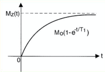
Fig 1. T1 relaxation

 Integrated Magnetic Resonance Centre for Doctoral Training, 8 Mar 2012, Retrieved from https://warwick.ac.uk/fac/sci/physics/research/condensedmatt/imr_cdt/students/stephen_day/relaxation/

Energy is not only loss from the interaction of spins with matter; precessing nuclei gradually fall out of synch with each other and stop producing a signal; this is called spin-spin relaxation.

 T₂ is then a time constant characterizing the signal decay to 37% of original (1/e)

The decay of magnitude can then be defined as

M⃗ xy(t) = M⃗ xy(0)e−t/T2

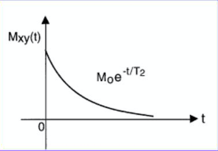
Fig 2. T2 relaxation

Integrated Magnetic Resonance Centre for Doctoral Training, 8 Mar 2012, Retrieved from https://warwick.ac.uk/fac/sci/physics/research/condensedmatt/imr_cdt/students/stephen_day/relaxation/

Spin-spin relaxation is essentially caused by inhomogeneities of the external magnetic field, and inhomogeneities of the local magnetic fields within the tissues.

The Bloch equations are the equations of motion of nuclear magnetization. They calculate nuclear magnetization M=(Mx,My,Mz) as a function of time while considering T1 and T2.

M is as discussed, a vector rotating in space, so it can be decomposed into three components, Mx(t), My(t), the transverse components, and Mz(t), the longitudinal component. (5)(6)

After a 90°-pulse and return to equilibrium the equations of motion can be simplified to

M_x(t) = M_o e ^−t/T2 sin ωt

M_y(t) = M_o e^−t/T2 cos ωt

M_z(t) = M_o (1 − e^−t/T1)

These equations demonstrate that there is will be a decay of the tranverse components back to zero and a reformation of the longitudinal component back to M0. M will precess around B in a spiralling fashion at the Larmor frequency.

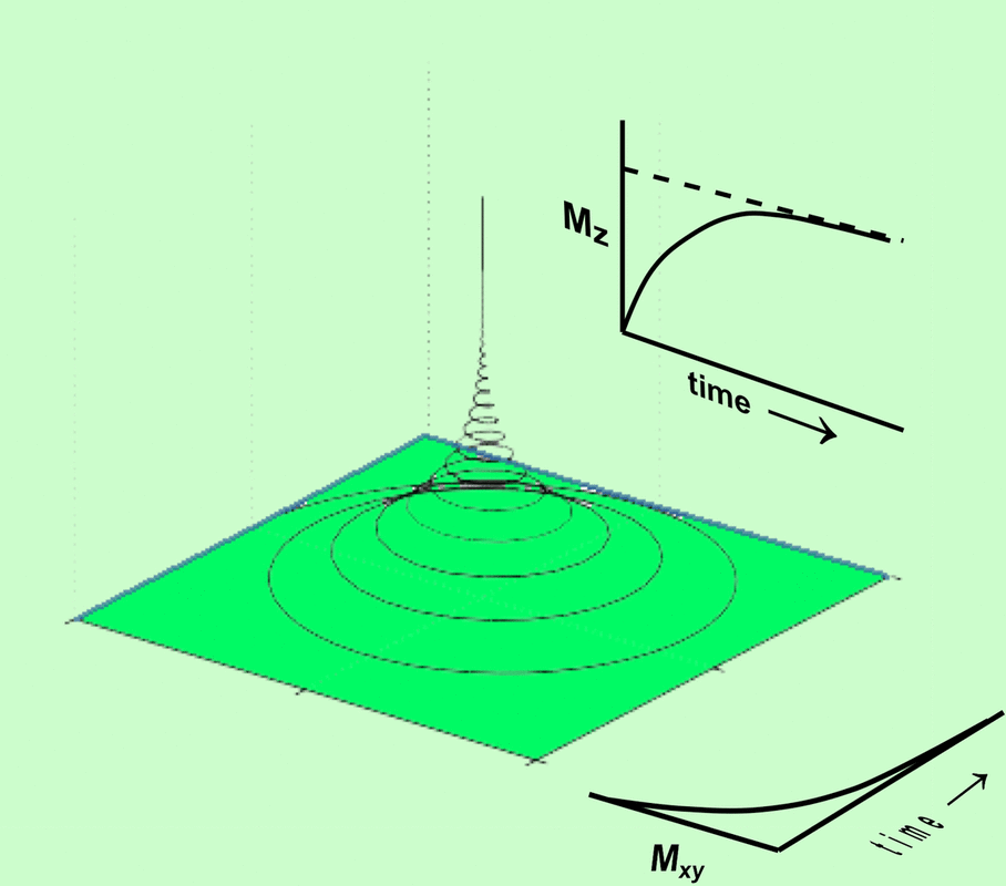
Fig 3. M exhibits precession in a spiral around B at the Larmor frequency

AD Elster, 2018 retrieved from http://mriquestions.com/bloch-equations.html

5. Pulse sequences

As mentioned before, MRI signal is essentially a manifestation of Faraday’s Law of Induction, where a changing magnetic field- in this case the net magnetization M during resonance-induces voltage in a conductor.

$\mathit{emf}= –\frac{\mathit{d\varphi }}{\mathit{dt}}$

Where $\mathit{d\varphi }$

is flux through the detecting coil.

MRI signal is a sine wave that oscillates at the Larmor frequency (ω_o)- we can classify NMR signal into free induction decay or echo (gradient echo, spin echo, stimulated echo).

Free Induction Decay arises after a single RF pulse and is a damped sine wave that results from the fact that the initially coherent transverse components of M dephase due to T2* decay.

T2* can be defined as encompassing T2 mechanisms and markedly field inhomogeneities, so can be regarded as an “effective T2”

FID is mathematically represented by

[sin ω_ot ] e^-t/T2*

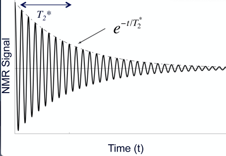
Fig 4. Free induction decay

Buxton R, The physics of functional magnetic resonance imaging (fMRI),
Reports on Progress in Physics, Volume 76, Number 9, 2013 IOP Publishing Ltd

The spin echo sequence consists of an initial 90° pulse, after which the isochromats dephase owing to field inhomogeneities, followed by a one or more 180° pulses neutralizes field inhomogeneities, which refocuses the spins – an echo results.

Two crucial variables in spin echo sequences are repetition time (TR), interval from the application of an excitation pulse to the application of the next pulse and echo time (TE), interval between the application of the radiofrequency excitation pulse and the peak of the signal induced in the coil, the centre of the echo.

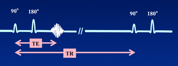
Fig 5. Spin echo, TE and TR

AD Elster, 2018 retrieved from http://mriquestions.com/se-vs-multi-se-vs-fse.html

These variables are used to manipulate image contrast; the combination of short TR and short TE gives a T1 weighted image while the combination of a long TR and a long TE gives a T2 weighted image.

A TR of less than 500 msec is considered short, a TR of more than 1500 msec long while A TE of less than 30 msec is considered to be short, a TE greater than 80 msec to be long.

Gradient echo (GRE) utilizes a frequency-encoding gradient twice: initially it applies a dephasing gradient that results in accelerated dephasing of the FID signal as it changes local magnetic fields and alters the resonance frequencies. A rephasing gradient- in essence a readout gradient- of the same strength but opposite polarity is subsequently applied and this re-aligns the dephased protons and acquires signal.

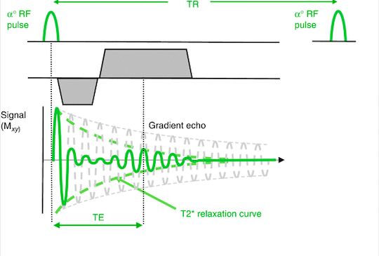
Fig 6. Gradient echo

Ridgway J.P. (2015) Gradient Echo Versus Spin Echo. In: Plein S., Greenwood J., Ridgway J. (eds) Cardiovascular MR Manual. Springer, Cham

Diffusion-weighted (DW) sequences are based on pulsed gradient spin echo (PGSE); Symmetric, strong diffusion-sensitizing gradients (DG’s) are applied on either side of the 180°-pulse.

The inversion recovery sequence applies a 180° pulse that turns the longitudinal magnetization in the opposite direction. This is followed by 90° and 180° pulses; essentially, it can be thought of as a conventional spin echo preceded by a 180° pulse.

The time between the 180°- and the 90° pulse is called TI = inversion time. After the initial 180° the longitudinal magnetization grows towards the +z-direction as the tissues undergo T1 relaxation. This aims to separate the longitudinal tissue magnetizations according to T1 relaxation times before application of the 90° pulse. As is true for spin echo, manipulation of TR and TE yields other contrast effects. IR is particularly utilized in cardiac imaging and neuroradiology (STIR, FLAIR).

Fig 7. Conventional Inverse Recovery sequence

Bitar R et al MR pulse sequences: what every radiologist wants to know but is afraid to ask, Radiographics. 2006 Mar-Apr;26(2):513-37.

6. From signal to image

In an MRI scan each voxel generates its own MR signal, and the technology depends on discerning where each signal is coming from to construct a meaningful image.

There are three steps involved in identifying where a signal is originating from in a 3D

a) Slice selection along z-axis

b) Segment of slice along x-axis selection by frequency encoding

c) Part of segment along y-axis selection by phase encoding

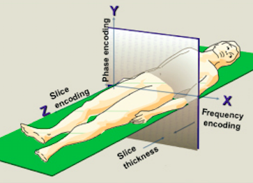
Fig 8. Spatial encoding in MRI

Fuster V et al, Hurst’s the Heart, 13^th edition, The McGraw-Hill Companies, 2011

Slice selection isolates a single plane in the object being imaged.

Slice selection is done by superimposing a gradient field – the slice selecting gradient- to the external magnetic field, along an axis orthogonal to the plane of the intended slice. Protons along this gradient field experience differential magnetic field strengths, showcasing different precession frequencies. The second step required for slice selection is applying an RF pulse that contains only those frequencies, and only the protons in the targeted slice will be excited and ultimately produce an image.

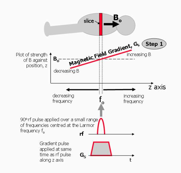
Figure 9. Slice selection

Ridgway J, Cardiovascular magnetic resonance physics for clinicians: Part I, Journal of Cardiovascular Magnetic Resonance 12(1):71 · November 2010

Slice thickness can be selected by altering the steepness of the gradient field or modifying the band width of the RF pulse. In practice, RF is not only one specific frequency, but a pulse in a range of frequencies; the width of the range of frequencies is directly proportional to the slice thickness, simply because more protons will be excited.

To locate a signal within a slice two other gradients are used, the frequency encoding gradient, which is applied after the slice selection gradient, and the phase encoding gradient.

The frequency encoding gradient acts within a slice and is applied along the y-axis. It mildly distorts the external magnetic field, resulting in differential Larmor frequencies along the y-axis and therefore differential frequencies of the signals produced. However, the frequency encoding gradient alone cannot discriminate between pixels in the same column as their frequencies are equal; phase encoding is concomitantly used to allow spatial detection.

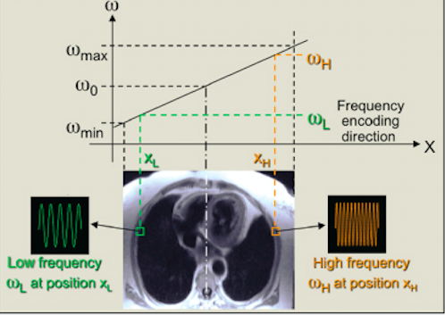
Fig 10. Frequency encoding

Plein S et al, Making an Image: Locating and encoding signals in space, Cardiovascular MR Manual, pp 43-55, Springer International Publishing

The phase encoding gradient is applied along the x-axis for a short time after the RF pulse; the protons along the x-axis precess with different frequencies.

When this gradient is switched off, the protons return to the initial precession frequency, which was equal for the whole population of spins; however, their signals are now out of phase, as they will have gained or lost phase relative to the reference state, and they demonstrate a permanent phase shift, which is detected and used for spatial encoding.

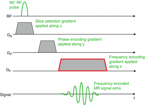
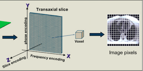
fig 11. signal localization in MRI

Plein S et al, Making an Image: Locating and encoding signals in space, Cardiovascular MR Manual, pp 43-55, Springer International Publishing

After applying the above described gradients, the outcome is a mixture of different signals with various frequencies vary; signals with the same frequency have different phases, which characterize their location. It is important to note that signal undergoes demodulation– multiplication of signal by a sinusoid or cosinusoid with a frequency around ω0.

K-space is a matrix where MR signals are stored (5) or, more accurately, it stores the spatial frequencies- repetitions per distance- of the entire object, which correspond to the variations in brightness. K-space trajectory refers to the manner in which k-space is populated; common trajectories are cartesian, spiral and radial.

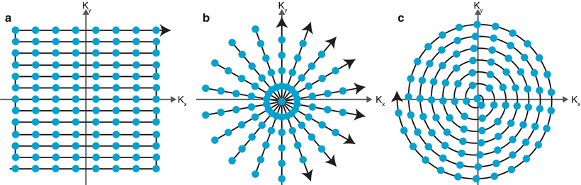
Fig 12. k-space trajectories from left to right, cartesian, radial, spiral

Syed MA et al (eds.) Basic Principles of Cardiovascular MRI: Physics and Imaging Technique, Springer International Publishing 2015

The brightness of a location in k-space represents the contribution of that specific spatial frequency to the image.

The edges of k-space tend to have high spatial frequency information; higher spatial frequency yields resolution/detail information while the centre of k-space contains lower spatial frequency and provides contrast information.The complex MRI signal is dismantled by the Fourier transformation and entered into k-space (8). A Fourier transform is an operation which converts a signal s(t) in the time domain to a complex number s(w) in the frequency domain. It decomposes the MR signal into a sum of sine waves with differing frequencies, phases and amplitudes. The inverse Fourier transform of each pixel in k-space contributes a specific signal 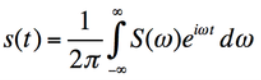frequency to the entire image.

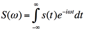
Fig 13 Fourier transform and inverse Fourier transform

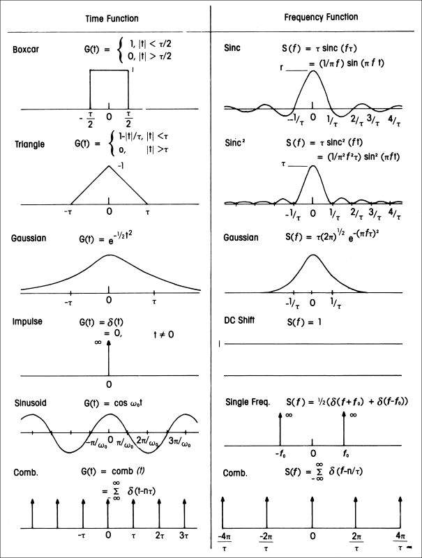
Fig 14. Fourier pairs

Sheriff, R. E. and Geldart, L. P., 1995, Exploration Seismology, 2nd Ed., Cambridge Univ. Press.

According to the shift theorem, a delay in the time domain corresponds to a linear phase term in the frequency domain, linear phase term meaning that its phase is a linear function of frequency.

Some of the information in k-space is redundant; k-space possesses a mirrored property

known as Hermitian symmetry and assuming no phase errors occur during data collection,

partial Fourier imaging techniques can be used to generate entire MR images from as little

as one-half of k-space.

The convolution theorem is central to Fourier theory application to image processing, the relationship being simply convolution in the time/space domain corresponds to multiplication in Fourier domain.

A practical example of this is smoothing an image with a Gaussian kernel, which can be done by computing the FT of the image and of the Gaussian kernel, multiplying their FTs, and lastly computing the inverse FT of product.

Convolution thus allows for filtering in MRI; we can define filters as low pass or high pass.

Low pass filters remove the high spatial frequency data from the periphery of k-space, while allowing low spatial frequencies to pass. The results is attenuation of image detail, although the coarse contrast of the image remains; they are useful for removing noise.

High pass filters on the other hand removes the low spatial frequencies, while allowing high spacial frequencies through. The latter are contained in the peripheries of k-space, and they represent the fine details of the image such as borders and, therefore, edges are enhanced.

7. References

1. Budinger T, Bird M, MRI and MRS of the human brain at magnetic fields of 14 T to 20 T: Technical feasibility, safety, and neuroscience horizons; NeuroImage, Volume 168, March 2018, Pages 509-531
2. Budinger T et al, Toward 20 T magnetic resonance for human brain studies: opportunities for discovery and neuroscience rationale; Magnetic Resonance Materials in Physics, Biology and Medicine, June 2016, Volume 29, Issue 3, pp617–639
3. Hanson L, Is quantum mechanics necessary for understanding magnetic resonance? Concepts Mag Reson Part A 2008;32A(5):329-340
4. Rigden JS. Quantum states and precession: the two discoveries of NMR. Rev Mod Physics 1986;58(2):433-448
5. Bloch F. Nuclear induction Phys Rev 1946;70:460-474,1946
6. Bloch F, Hansen WW, Packard M. The nuclear induction experiment. Phys Rev 1946;70;474-485
7. Moratal D,Vallés-Luch A, Martí-Bonmatí L, Brummer M. k-space tutorial: an MRI educational tool for a better understanding of k-space. Biomed Imaging Interv J. 2008;4(1): e15.
8. Gallagher TA, Nemeth AJ, Hacein-Bey L. An introduction to the Fourier transform:relationship to MRI. AJR Am Roentgenol 2008; 190:1396-1405.
9. McRobbie D, Moore E, Graves M, Prince M (2006). MRI from Picture to Proton. Cambridge: Cambridge University Press.