Mathematical Modeling of Disease Epidemics
| ✅ Paper Type: Free Essay | ✅ Subject: Sciences |
| ✅ Wordcount: 3533 words | ✅ Published: 23 Sep 2019 |
MATHEMATICAL MODELING OF DISEASE EPIDEMICS
GISELLE RASQUINHA
INTRODUCTION:Throughout history we have seen pandemic diseases such as the bubonic plague that swept through the Middle Ages in Europe and the Spanish Flu at the beginning of the 20th century (Scientific American, 2008). In the last 50 years, we have seen HIV responsible for millions of deaths. There have been health scares over bird flu, SARS and Ebola – yet none of these diseases developed into a major global health problem. Many diseases such as the common cold, are have an inconsequential effect; but others, such as those caused by Ebola virus or the HIV virus, raise panic. The seemingly random victim that the disease picks is what makes people filled with dread. However, diseases are an inevitable part of our life and to remove some of the uncertainty associated with infection, mathematics can be used to both understand how diseases spread and then predict future movements of the disease, thus relating important epidemiology questions to the basic characteristics of infection (Keeling, 2001). Additionally, immunization is a powerful tool that allows for prevention of infection at a population level rather than treating the disease symptoms. This permits a higher level of prediction regarding the spread of infections (Scherer and MacLean, 2002). In this paper, I shall focus on the most basic of disease models and also take into account some of the more mathematical advances that have increased our ability to predict where, how and to whom the disease can spread, by focusing on the utility of mathematical modeling in public health and then to understand the impact of immunization at the population level.
MATHEMATICAL MODELING OF INFECTIOUS DISEASES: The mathematics of disease is a data−driven subject. The main aim of this field of research is to link mathematical models and disease data. Reports of disease cases can be obtained from doctors to yield a highly detailed sources of important data relating to that specific disease including the number of weekly disease cases for a variety of populations over multiple years. This data will be modified by changes in birth or death rates and parameters like increased social contacts during the school year and is termed the signature of social effects (IB Math Resources, May 2014). Therefore, to create a comprehensive picture of disease dynamics we need a variety of mathematical tools, including design of a mathematical model that is based on both differential equations and statistical analysis.
HOW CAN MATHEMATICAL MODELS HELP? Models help in the understanding of the transmission of infections in a population, to interpret observed epidemiological trends, to identify key determinants of epidemics, to guide the collection of data, to forecast the future direction of an epidemic and to evaluate the potential impact of an intervention (Keeling, 2001). Using mathematical tools to model the spread of diseases is one of the main ways of preparing for potential new disease epidemics. Besides providing information to physicians about the levels of immunization that will be required to keep a population disease-free, it also helps decide what first response actions are needed when new diseases emerge on a global scale (for example, H1N1 flu, SARS viral diseases and Ebola)
THE BEGINNINGS OF MATHEMATICAL EPIDEMIOLOGY: There were four major players that laid the foundation of the mathematical epidemiology field. The very first scientist was Daniel Bernoulli who in 1760 formulated and solved a model for smallpox. Using his model, he evaluated the effectiveness of inoculating healthy people against the smallpox virus. The second major contributor was Hamer. In 1906 Hamer formulated and analyzed a discrete time model to understand the recurrence of measles epidemics. Ronald Ross developed differential equation models for malaria as a host-vector disease in 1911. Ross was awarded the Nobel Prize in Medicine for his work on modeling. Lastly Kermack and McKendrick obtained epidemic threshold results by extending Ross’s models in 1926.
TYPES OF MODELS (Mishra, 2011): There are two basic categories of models in use for disease epidemiology-Deterministic or compartmental and Probabilistic or stochastic models. A deterministic model is one where elements of randomness are not built in. Whenever the model is run with identiacl initial conditions you will get the same results. Results imply epidemic will always take same course, which is not always true. However, a probabilistic model Incorporates the role of chance and variation in parameters and can thus provide a range of possible outcomes. The deterministic model is also called the compartmental model because it describes transitions between compartments by applying average transition rates. It Aims to describe what happens “on average” in a population. The probabilistic model is particularly relevant for small populations and used early in epidemics. In this paper, I will focus on the most basic compartmental model-the SIR model.
SIR MATHEMATICAL MODEL OF DISEASE : (Smith and Moore, 2004) Most mathematical models describing the spread of disease begin using the same assumption: that the population can be compartmentalized into groups, described by their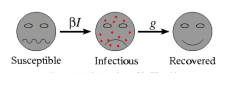
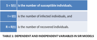
exposure to the disease. The most basic of these mathematical models, categorizes individuals as belonging to one of three categories-susceptible, infectious or recovered. This model is known as the SIR model (represented by the picture above, Fig 1). To begin the mathematical modeling process, we identify the two variables-independent and dependent. The independent variable is “t” which stands for time and is always measured in days (Table 1). We next consider two sets of dependent variables: The first set of dependent variables calculates and sums people in each of the groups, each as a function of time: The next set of dependent variables is related to the first and corresponds to the fraction of the total population in each of the three groups. So, if N is the total population, we have fractions of population as represented in Table 2. The SIR model examines the fraction of the population that is susceptible to infection, how many of these go on to become infectious, and how many of these go on to recover (and in what timeframe). There are several assumptions in this model. The population is fixed, no entries (births) or exits (deaths). All newly born individuals enter the susceptible class. Disease-susceptible individuals are considered naïve and have never interacted with or been exposed to the disease and are able to catch the disease. At this point, they will transfer into the infectious class. These individuals are responsible for spreading the disease to the susceptible class, and these individuals stay in the infectious class for a set period of time, that is specific to the disease, called the infectious period, before moving into the recovered class. The last assumption of the model is that all subjects in the recovered category are assumed to be immune for their life-spans.
DIFFERENTIAL EQUATIONS IN REAL LIFE: This description of the various categories of infection can be made more mathematical by designing a mathematical equation, called a differential equation, for the ratio of individuals in each class. Differential equations have a significant ability to predict the world around us (IB Maths Resources, Feb 2014). Applications of these equations have been exploited in a large number of scientific and economic fields, ranging from population biology to economics and engineering. The utility of these equations arises from the fact that they can define exponential growth and decay, the growth of species of different animals and plants or even in the stock market to describe the change in investment return over time. A differential equation is a mathematical equation that contains variables like x or y, and describes the rate at which these variables change. The unique features of differential equations arise from the fact that their solutions are functions instead of numbers. A differential equation generally is written in the form dy/dx = ………. Some differential equations can be simply solved (to get y = …..) by simple integration, while others require complex mathematics. Although a precise solution can be obtained for some differential equations, it is not possible to solve many equations exactly, as their solutions can only be estimated. This is where computer programs are exploited to supply precise solutions to these equations at a much faster speed..
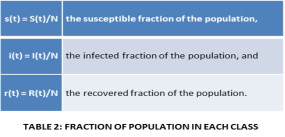
DIFFERENTIAL EQUATIONS AND APPLICATIONS TO MODELLING: (Smith and Moore, 2004) The population of individuals that are susceptible to the disease will decline over the course of the epidemic as new individuals becom
e infected. If no new people enter the population via birth or immigration, there is no way to generate additional susceptible individuals in this model. If we assume random encounters among individuals, then contacts between infected and susceptible individuals will be proportional to the product S*I. Thus, the rate of change that will be measured in all 3 populations (S, I and R) is shown in Fig 2, where β is the probability of transmission for each contact between infected and susceptible persons, c is the contact rate and D is the duration of infectivity. This population of infected people will increase as new infected cases develop (will occur at a rate +βcSI) and decrease as infected individuals recover (at a rate of I/D). Recovery from the disease subtracts individuals from the infected pool at rate I/D. The sum of S+I+R=1.0, thus we only track two classes (and then calculate the amount of people in the third class) (Stratton, 2010). Let us look at specific scenarios, if dI/dt is high this signifies that the number of people that are getting infected is increasing at a high rate. When dI/dt is zero this signifies that there is no difference in the numbers of people becoming infected (number of infections remain constant). When dI/dt is negative then the numbers of individuals developing infections is decreasing. The constants β, c and D are disease- specific and will vary depending on the disease being modelled.
The Epidemiological Parameter R0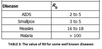 : R0 is the basic factor that dictates the spread of diseases. Additionally, it is also related to how the disease will fare in the future and the level of immunization or vaccination necessary for eradication. This parameter is called the basic reproductive ratio R0. It is defined by epidemiologists as “the average number of secondary cases caused by an infectious individual in a totally susceptible population” (Kucharski, 2014). R0 describes the initial rate of increase of a specific disease over a generation. In cases where R0 >1, the disease can sicken a totally susceptible population and the number of cases will increase. If R0 <1, the disease agent will always fail to spread. Therefore, in its most basic form, R0 describes whether a population is at risk from a given disease. The R0 values for different diseases ranging from AIDS to malaria are shown above and underlines why specific diseases are highly infectious, how because it is an airborne disease, measles is can spread quickly – and how malaria is a difficult disease to control because infected people act like a storage bank for the parasites that live inside the vector mosquitoes.
Determinants of R0 and application to epidemic modelling:For any disease-causing agent that requires direct person-to-person transmission, R0 can be calculatedas:
R0 = βcD (where β is the probability of transmission per contact between infected and susceptible persons, c is the contact rate and D is the duration of infectivity).
Epidemiologists generally focus on these big questions for epidemics: Under what conditions will that specific disease spread? (When is dI/dt>0)? When will the specific infection stop growing (dI/dt=0) (when the epidemic is over)? What proportion of the population will acquire the disease? Under what conditions will the disease spread?
dI/dt =0 when I =0 (the disease is not present)
or when βcS=1/D.
Rearranging S =1/βcD (Stratton, 2010).
That means that we can define and enumerate a critical proportion of susceptible individuals that is required for an epidemic to take place. If S is less than that number, dI/dt< 0and this will ensure that the infection willdie out.Is it possible to reduce the number of susceptible individuals in the population and how?
HERD IMMUNITY: (Willingham and Helft,2014) The main route to prevent the spread of disease is to vaccinate individuals. If a high enough proportion of the population is vaccinated, then the epidemic will eventually die out, even in individuals that did not receive the vaccine. This is known as “herd immunity” (Figure 3). People who are not immunized can indirectly get protection if enough of the population get vaccinated. Herd immunity, is a condition in which most of a population is able to resist the cause of an infectious disease, and thus restricting the degree to which the infection can spread through the population. This community immunity can be obtained through different means, it can be acquired through natural immunity, earlier 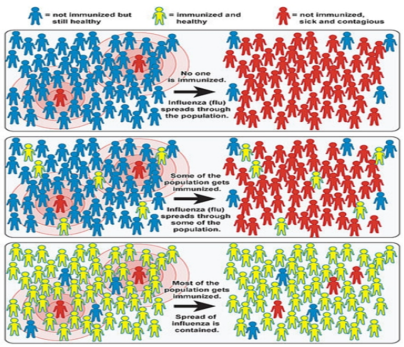
exposure to the disease, or immunization. The whole population does not require to be immune to attain herd immunity. Rather, herd immunity can occur when the population density of individuals who are susceptible to infection is adequately low to minimize the probability of interaction between an infected individual and a susceptible individual. Herd immunity can prevent persistent and chronic spread of the infection in populations, and thus protect susceptible individuals from infection. It is applicable, however, only to infectious diseases that are contagious through human contact. Each infectious disease will have its own defined proportion of the population that must be immune to produce herd immunity. Highly contagious pathogens, such as the measles virus, needs a much higher number of immune persons to achieve herd immunity status than a disease that is less infectious, such as tuberculosis. In addition, criteria that operate at both the individual and population level like susceptibility, demographics, and social habits can influence the spread of disease also have an impact on herd immunity.
Figure 3: Illustration of the Impact of Herd Immunity on Infection Rates (Sc. American, 2008)
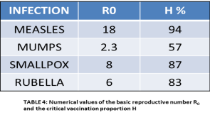 MATHEMATICAL RELATIONSHIP BETWEEN R0 AND HERD IMMUNITY: (Scherer and McLean, 2002) Herd immunity is one of the critical parameters epidemiologists consider for mass vaccination practices. Even if a cheap, safe, and effective vaccine exists, resource, logistical, and societal constraints can prevent the vaccination of 100 percent of the population (Willingham and Helft, 2014). Therefore it is important to define a target level of vaccination to achieve the threshold level of herd immunity (H). It can be calculated as
H > 1 − 1/R0,
where R0 is the basic reproductive rate (Keeling, 2001). Vaccination of a large proportion of the population can be successful through principles of herd immunity to ensure that both the occurrence and the severity of disease outbreaks that may occur are reduced, if not eliminated.
MODELING MEASLES: (IB Math Resources, May 2014). With measles we have an average infection of about a week, (so if we want to work in days, D=7) and R0 = 15 then
R0 = βcD 15 = βc7 βc = 2.14
Using these values, we can formulate 3 equations for rates of change:
dS/dt = -2.14 I S
dI/dt = 2.14 I S – 0.14 I
dR/dt = 0.14 I
Unfortunately all modeling equations are very difficult to solve. However, computer programs exist that allow us to plot different epidemic conditions specific for different diseases using disease specific parameters. If we identify starting values for S, I and R, which correspond to the numbers of susceptible, infectious, recovered (immune) individuals from measles, we can plug them in to predict how it will spread. In the first case, let us assume that total population is made of 11 people, of these 10 individuals are susceptible to measles, 1 has the measles virus and none (0) who are immune to the disease. The expected result for disease spread is shown in Fig 4A. The graph depicts that the virus spreads very quickly and by the second day, 8 people come down with the measles virus. The majority of the population does not succumb to the disease and are said to have become immune by day 10. However, the disease is still in the
Figure 4: Computer Modeling of Measles
A: Small Population, No immunity
B: Large Population, No immunity
C: Large Population, Herd immunity
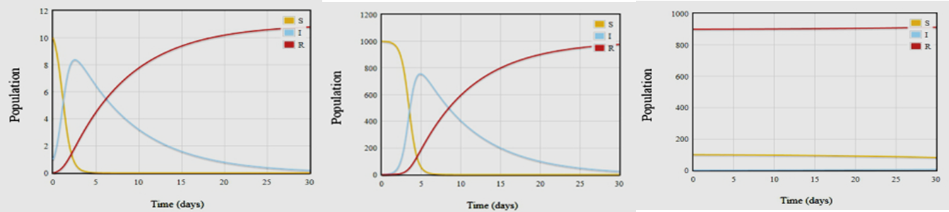
Population. In a month, at day 30, everyone in the population has achieved immunity and the measles infection has died out. A depiction of just how quickly measles can spread is provided by Figure 4B. For this example, our initial population size is1000 people with only 1 case of measles infection. Despite this low level of starting infection, in less than a week, approximately 5 days, we find that > 75% of the population get sick with the measles virus. The power of herd immunity is illustrated in Fig. 4C. For this example, we assume that there are100 people who are susceptible to the virus, but there are 900 people who have had the virus and are recovered and therefore considered immune to the virus. In this population, there is one infectious person. As can be seen from the graph in Fig 4C, the measles virus cannot find a foothold in the population as the immune individuals act as a safeguard against infection.
LIMITATIONS OF THE SIR MODEL: There are many assumptions that the SIR model makes, that limit its applicability- first that the total population size remains constant, with no births or deaths resulting in changes to the numbers. It also assumes that the population is uniform and homogeneously mixing. Mixing depends on many factors including age. Contact rates among individuals will differ depending on geographical locations as well as the social-economic groups to which they belong. The model ignores random effects, which can be very important when “s” or “i” are small, which are common features during the initial stages of the epidemic.
CONCLUSIONS: In the battle against disease, the difference between an infection that causes a raging epidemic and a short-term fever comes down to one parameter-R0. The reproduction number is critical because it encapsulates all the key features of disease transmission, from social behavior to degree of infection, into a single parameter. The size of this parameter can be used to predict what will happen during an epidemic (Kucharski, 2014). The major advantage of mathematical approaches to disease modeling is its ability to make such predictions about the spread of disease during epidemics. It is useful to model and understand how disease dynamics change for multiple reasons: it is important for basic science as well as for public policy.
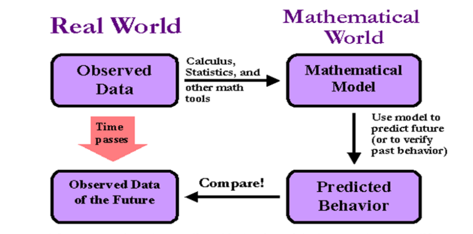
Figure 5: Applications of Mathematical Models in the Real World
Modeling of infectious diseases is helpful for prevention and control of emerging diseases like SARS and Ebola. Using models, we do not have to use the real-world scenarios but can test control strategies by using models (Figure 5). Multiple treatments and interventions can be compared against each other before they are put into practice. Potential control measures can also be decided by regarding epidemics as dynamic. For example, we can ask are there any scenarios in which vaccines should be targeted to certain groups or whether there are scenarios in which the predicted epidemic will exceed medical capacity. Mathematical models of various levels of complexity can thus be exploited to reap the greatest public-health benefit.
BIBLIOGRAPHY
- “Differential Equations in Real Life.” IB Maths Resources from British International School Phuket, 13 Feb. 2014.
- “Infectious Diseases: A Scientific American Reader.” University of Chicago, 2008.
- Keeling, Matt. “The Mathematics of Disease.” Plus Magazine, University of Cambridge, 1 Mar. 2001.
- Kucharski, Adam. “The Calculus of Contagion.” 16 Sept. 2014.
- Mishra, S., et al. “The ABC of Terms Used in Mathematical Models of Infectious Diseases.” Journal of Epidemiology & Community Health, vol. 65, no. 1, 2010, pp. 87–94., doi:10.1136/jech.2009.097113.
- “Modelling Infectious Diseases.” IB Maths Resources from British International School Phuket, 13 Feb. 2014.
- Scherer, Almut, and Angela Mclean. “Mathematical Models of Vaccination.” British Medical Bulletin, vol. 62, no. 1, Jan. 2002, pp. 187–199., doi:10.1093/bmb/62.1.187.
- Smith, David, and Lang Moore. “The SIR Model for Spread of Disease – The Differential Equation Model.” Journal of Online Mathematics and Its Applications, Mathematical Association of America, Dec. 2004.
- Stratton, Don. “The Population Biology of Infectious Disease.” Case Studies in Ecology and Evolution, June 2010.
- Willingham, Emily, and Laura Helft. “What Is Herd Immunity?” PBS, 9 May 2014.
Cite This Work
To export a reference to this article please select a referencing stye below:
Related Services
View all


DMCA / Removal Request
If you are the original writer of this essay and no longer wish to have your work published on UKEssays.com then please click the following link to email our support team:
Request essay removal