Experiment of the Characteristics of an Orifice Plate Meter

Orifice Plate Report

Abstract

An experiment was conducted to explore the characteristics of an orifice plate meter. This was done using a Cussons hydraulic flow bench. Eight sets of readings were obtained for the measured manometer readings from the four tappings and the inlet tank and outlet tank. The flow rate was also obtained by collecting five litres of water and timing the length of time it required. A couple of the sets of readings appeared to be abnormal so they were repeated. This experiment was done to acquire the values of the coefficient of discharge. From the obtained results, two methods of calculations could be used to calculate the value of the coefficient of discharge, one for a theoretical value and one for an experimental value. The findings of this experiment are that the flowrate affects the coefficient of discharge, the lower the flow rate the higher the coefficient of discharge. If the pressure tappings were put at a different location, then it was found that the flow rate barely affected the coefficient of discharge.

Introduction

The experiment was conducted using a Cussons hydraulic flow bench.

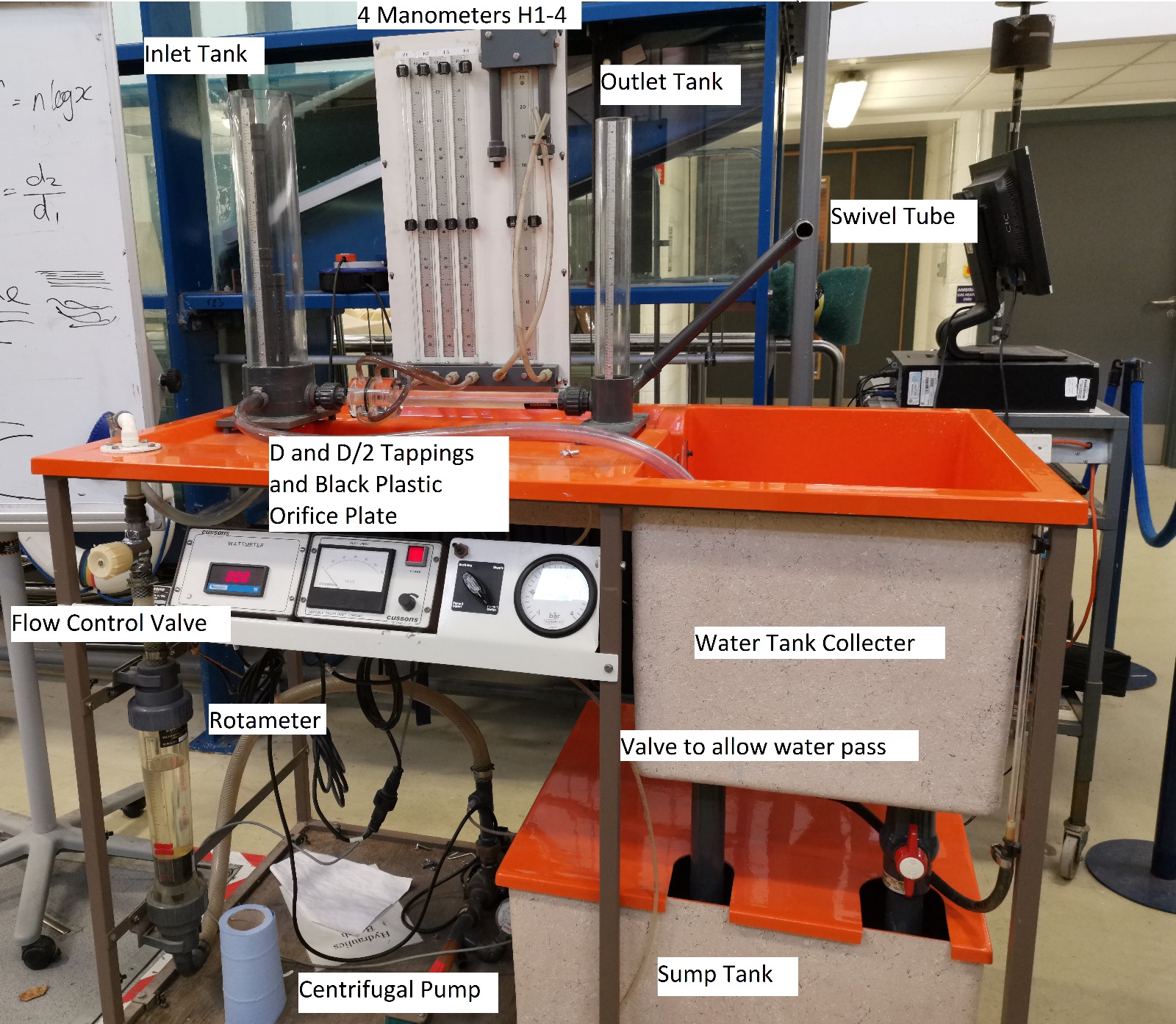
Figure 1 – A Photo of the Experiment setup

Method

• The flow control valve is opened until the inlet tank is about 498mm.
• The swivel tube is raised until the outlet tank is about 225mm.
• Readings of the four manometers H1-4 are recorded.
• The valve to allow water pass is turned to collect water. This is timed using a stopwatch until five litres is collected and the valve is turned back.
• Raise the swivel tube so that the outlet tank is increased by about 20mm.
• Repeat all steps

The tappings used were D and D/2 tappings.

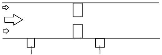
Figure 2 – A Diagram of D and D/2 Tappings

Equations

$Q=\frac{V}{1000\times t}$

Where:

Q = Flow Rate (m³/s)

V = Volume (m³)

t = time (s)

Time is multiplied by 1000 as the volume recorded from the experiment is in litres rather than m³.

$∆H_1=\frac{(H2–H1)}{1000}$

Where:

$∆H_1$

= Head loss at corner tappings (m)

H2 = Head at manometer 2 (mm)

H1 = Head at manometer 1 (mm)

$∆H_2=\frac{(H4–H3)}{1000}$

Where:

$∆H_2$

= Head loss at D and D/2 tappings(m)

H4 = Head at manometer 4 (mm)

H3 = Head at manometer 3 (mm)

${\log }_{10}Q$

Where:

Q = Flow Rate (m³/s)

${\log }_{10}∆H_1$

Where:

$∆H_1$

= Head loss at corner tappings (m)

${\log }_{10}∆H_2$

Where:

$∆H_2$

= Head loss at D and D/2 tappings(m)

$\beta =\frac{d_2}{d_1}$

Where:

$\beta$

= Diameter Ratio

d₂ = Diameter of Orifice (m)

d₁ = Pipe Bore (m)

$C_d= \frac{{10}^C}{A_2}{\left[\frac{1–{\beta }^4}{2g}\right]}^{\frac{1}{2}}$

Where:

C_d = Coefficient of Discharge

c = y-intercept from graph

A₂ = Area of orifice (m²)

$\beta$

= Diameter Ratio

g = Gravity (ms^-2)

This equation is for the theoretical value of coefficient of discharge.

$R_{e_d}=\frac{\rho \times v\times d}{\mu }$

Where:

$R_{e_d}$

= Reynolds Number

$\rho$

= Density (kg/m³)

v = Velocity (ms^-1)

d = Pipe Bore (m)

$\mu$

= Viscosity (kg/ms)

$C_d=0.5959+0.0312{\beta }^{2.1}–0.184{\beta }^8+0.0029{\beta }^{2.5}{\left(\frac{{10}^6}{R_{e_d}}\right)}^{0.75}+\frac{0.039{\beta }^4}{\left(1–{\beta }^4\right)}–0.015839{\beta }^3$

Where:

C_d = Coefficient of Discharge

$\beta$

= Diameter Ratio

$R_{e_d}$

= Reynolds Number

This equation is for the experimental value of coefficient of discharge for orifice plates with D and D/2 tappings.

$C_d=0.5959+0.0312{\beta }^{2.1}–0.184{\beta }^8+0.0029{\beta }^{2.5}{\left(\frac{{10}^6}{R_{e_d}}\right)}^{0.75}$

Where:

C_d = Coefficient of Discharge

$\beta$

= Diameter Ratio

$R_{e_d}$

= Reynolds Number

This equation is for the experimental value of coefficient of discharge for orifice plates with corner tappings.

$A=\frac{\pi d^2}{4}$

Where:

A = Area (m²)

d = diameter of circle (m)

$v=\sqrt{\frac{2g∆H}{1–{\beta }^4}}$

Where:

v = Velocity (ms^-1)

g = Gravity (ms^-2)

β = Diameter Ratio

$∆H$

= Use $∆H_1$

for corner tappings and $∆H_2$

for D and D/2 tappings

Experiment Results

Figure 3 – Table of Results from Experiment

All sample calculations shown below will be used using the first set of results.

$Q=\frac{5}{1000\times 20.2}=0.0002475$

$∆H_1=\frac{(465–96)}{1000}=0.369$

$∆H_2=\frac{(465–100)}{1000}=0.365$

${\log }_{10}Q={\log }_{10}0.0002475=–3.606$

${\log }_{10}∆H_1={\log }_{10}0.369=–0.4330$

${\log }_{10}∆H_2={\log }_{10}0.365=–0.4377$

Figure 4 – Table of Calculations

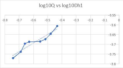
Figure 5 – Graph of log₁₀Q vs log₁₀ $\mathit{∆}{\mathit{H}}_{\mathit{1}}$

From figure 5 it can be found that the gradient, m, is 0.4418 and the y-intercept, c, is -3.4285.

d1 = 0.022m

d2 = 0.012m

$\beta =\frac{0.012}{0.022}=0.545$

$A_2=\frac{\pi {(0.012)}^2}{4}=1.131\times {10}^{–4}$

$\beta$

= 0.545

A₂ = $1.131\times {10}^{–4}$

m²

$C_d= \frac{{10}^{–3.4285}}{1.131\times {10}^{–4}}{\left[\frac{1–{0.545}^4}{2\times 9.81}\right]}^{\frac{1}{2}}=0.711$

The theoretical value of the coefficient of discharge is 0.711

$\rho$

= 1000 kg/m³

$\mu$

= 1.13×10^-3 kg/ms

$R_{e_d}=\frac{1000\times 0.029\times \sqrt{\frac{2\times 9.81\times 0.369}{1–{0.545}^4}}}{1.13\times {10}^{–3}}=54860.88$

Figure 6 – A table of Reynolds numbers for $\mathit{∆}{\mathit{H}}_{\mathit{1}}$

, corner tappings, and $\mathit{ }\mathit{∆}{\mathit{H}}_{\mathit{2}}$

, D and D/2 tappings

$C_d∆H_1=0.5959+0.0312{\beta }^{2.1}–0.184{\beta }^8+0.0029{\beta }^{2.5}{\left(\frac{{10}^6}{R_{e_d}∆H_1}\right)}^{0.75}$

$C_d∆H_1=0.5959+0.0312{(0.545)}^{2.1}–0.184{\left(0.545\right)}^8+0.0029{\left(0.545\right)}^{2.5}{\left(\frac{{10}^6}{54860.88}\right)}^{0.75}=0.609$

$C_d∆H_2=0.5959+0.0312{\beta }^{2.1}–0.184{\beta }^8+0.0029{\beta }^{2.5}{\left(\frac{{10}^6}{R_{e_d} ∆H_2}\right)}^{0.75}+\frac{0.039{\beta }^4}{\left(1–{\beta }^4\right)}–0.015839{\beta }^3$

$C_d∆H_2=0.5959+0.0312{(0.545)}^{2.1}–0.184{\left(0.545\right)}^8+0.0029{\left(0.545\right)}^{2.5}{\left(\frac{{10}^6}{54562.72}\right)}^{0.75}+\frac{0.039{\left(0.545\right)}^4}{\left(1–{0.545}^4\right)}–0.015839{\left(0.545\right)}^3=0.610$

Figure 7 – A table of experimental coefficient of discharge for $\mathit{∆}{\mathit{H}}_{\mathit{1}}$

, corner tappings, and $\mathit{ }\mathit{∆}{\mathit{H}}_{\mathit{2}}$

, D and D/2 tappings

Discussion

From the theoretical calculations, it was calculated that the coefficient of discharge is 0.71. From the experimental calculations, it was calculated that the coefficient of discharge is about 0.61. So, the experimental value is lower than the theoretical value and this is expected as the theoretical value is for ideal flow whereas the experimental value is affected by friction resulting in energy losses.

This experiment is easy to repeat and is not time consuming to do so. Although two of the sets were repeated due to abnormal data, the overall experiment was only done once and not repeated meaning that it is unknown whether the other six sets of data have any abnormal data. The accuracy of the results may vary as all of the recorded results had to be done manually, reading the manometer, opening and closing the valve, starting and stopping the stopwatch. All of these actions have human error especially the starting and stopping the stopwatch which required two people so there would be a delay in the actions and commands between them. The four manometers were held in place by a black rubber ring which covered the manometer at a certain point and one of the manometers got behind it meaning that we could not accurately read the value, so that value had to be guessed.

From Figure 7 it appears that the measured value of the coefficient of discharge remains consistent throughout the range of flow rates of 0.61. By comparing the coefficient of discharge values from the corner tappings and the D and D/2 tappings, using corner tappings it is shown that the value is 0.001 lower than the D and D/2 tappings, but it is clear that the location of the pressure tappings has negligible effect on the coefficient of discharge.

The plot log₁₀Q vs log₁₀ $∆H_1$

should be a straight line with gradient equal to 0.5 and from my graph, the gradient is 0.4418 which is close.

Using an orifice plate is a lot cheaper as the orifice plate itself can be manufactured from plastic and be easily replaced. This is also beneficial as the orifice plate may be worn down over time and changing it will be quick and easy. It is also easy to change the size of the orifice or use different hole shapes for different experiments. It is overall easier to fabricate the orifice plate than a venturi meter and requires less space. 

There are some disadvantages when the orifice plate is compared to a venturi meter. Due to the design of the orifice plate, the water flow in the pipe will experience a sharp corner resulting in the flow area of the vena contracta being smaller than the area of the orifice whereas in theory the flow area of the vena contracta should be the area of the orifice. This results in a large energy loss. The venturi meter’s design is a gradual slope from the diameter of the pipe to the diameter of the orifice allowing the water flow in the pipe to experience a smooth change resulting in the flow area of the vena contracta being the area of the orifice. This leads to a low or minimal energy loss. This means that the venturi meter will have a higher coefficient of discharge than the orifice plate and the results will be more accurate.

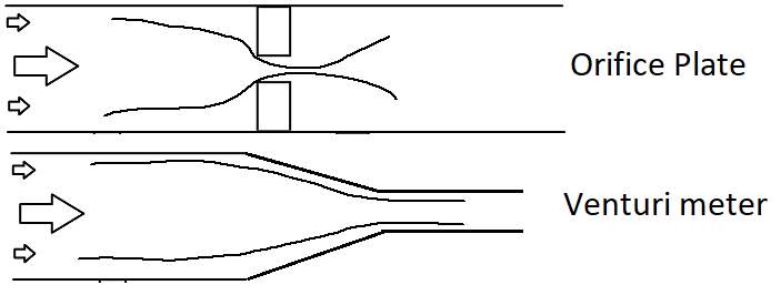
Figure 8 – Water flow in an orifice plate vs venturi meter

Conclusion

To conclude, from this experiment it has been found that the theoretical value, 0.71, and the experimental value, 0.61, of the coefficient of discharge is what was expected. The experimental value was expected to be lower due to it representing the actual flow rate and the theoretical value was expected to be higher as it represents the ideal flow rate. If this experiment were to be done again, it would be repeated again to eliminate the chances of abnormal data existing and to ensure that the results are consistent.

References

1. Figure 1 – A Photo of the Experiment setup
2. Figure 2 – A Diagram of D and D/2 Tappings
3. Figure 3 – Table of Results from Experiment
4. Figure 4 – Table of Calculations
5. Figure 5 – Graph of log₁₀Q vs log₁₀ $∆H_1$
6. Figure 6 – A table of Reynolds numbers for $∆H_1$

   , corner tappings, and $∆H_2$

   , D and D/2 tappings

7. Figure 7 – A table of experimental coefficient of discharge for $∆H_1$

   , corner tappings, and $∆H_2$

   , D and D/2 tappings

8. Figure 8 – Water flow in an orifice plate vs venturi meter