Analysis of Response Surface Methodology (RSM)
| ✅ Paper Type: Free Essay | ✅ Subject: Sciences |
| ✅ Wordcount: 3003 words | ✅ Published: 11 Apr 2018 |
1.3 DESIGN OF EXPERIMENTS 34, 35
Trans-Pacific Partnership economic framework agreement has clearly defined that many studies must be conducted to develop a formulation. Design of experiments (DOE) has proven to be an effective tool for formulation scientists throughout the many stages of the formulation process. At every step of formulation development, DOE can aid in making intelligent decisions. These steps include excipient compatibility studies, process feasibility studies, formulation optimization, process optimization, scale-up and manufacturing process characterization. Lastly, the product and manufacturing process must be validated before it is on the market.
The word optimize is defined as, making as perfect, effective or functional as possible. Optimization may be interpreted as to find out the value of controllable independent variable, that gives the most desired value of dependent variables. The application of formulation optimization techniques is relatively new to the practice of pharmacy when used intelligently, with the common sense, these “statistical” methods will broaden the perspective of the formulation process.
At the Preformulation stage, before any experiment is conducted certain problem arises, it is often not known before hand which variable will significantly influence the response. Screening designs and ANOVA helps to solve this problem.
A second serious complication may arise with new excipients and new process factor, for which qualitative or quantitative effects are not known and are unpredictable. The following questions must be answered before choosing any design of experiment.
The third complication is that formulated products, in particular dosage form has to confirm to several requirements, very often competing. The formulator has to trade off objectives and choose a compromise.
A fourth problem is the lack of insight` to perform an adequate optimization studies.
Above all in the performance of an optimization study, the formulation development scientist can also be a factor as personal variation.
1.3.1 Terms used in Design of experiments
Variables
These are the measurements, values, which are characteristics of the data. There are two types of variables; dependent variables and independent variables. Independent variables(X) are set in advance, which are not influenced by any other values e.g., Lubricants concentration, drug to polymer ratio, etc. Dependent variables(Y) are the outcome variables, influenced by the independent variables e.g., hardness, dissolution rate, etc.
Factor
Factor is an assigned variable such as concentration, temperature, lubricant agent, drug to polymer ratio, polymer to polymer ratio or polymer grade. A factor can be qualitative or quantitative. A quantitative factor has a numerical value to it for example, concentration (1%, 2%… so on), drug to polymer ratio (1:1, 1:2…etc). Qualitative factors are the factors, which are not numerical value, for example, the polymer grade, humidity condition, type of equipment, etc. these are discrete in nature.
Levels
The levels of a factor are the values or designation assigned to the factor. For e.g. in concentration (factor) 1 % will be one level, while 2% will be another level. Two different plasticizers are levels for grade factor. Usually levels are indicated as low, middle or high level. Normally for ease of calculation the numeric and discrete levels are converted to –1 (low level) and +1 (high level).The general formula for this conversion is
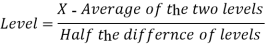
Where ‘X’ is the numeric value
Response
Response is mostly interpreted as the outcome of an experiment. It is the effect, which we are going to evaluate i.e. Disintegration time, duration of buoyancy, etc.
Effect
The effect of a factor is the change in response caused by varying the levels of the factor. This describes the relationship between various factors and levels.
Interaction
Interaction is also similar to effect, which gives the overall effect of two or more variables (factors) on a response. For example, the combined effect of lubricants (factor) and glidants (factor) on hardness (response) of a tablet.
In the trial and error method, a lot of formulations have to be prepared to get a conclusion, which involves lots of money, time and energy. These can be minimized by the use of optimization technique.
1.3.2 Optimization Process
Generally optimization process involves the following steps.
- Based on the previous knowledge or experience or from literature, the independent variables are determined and set in the beginning.
- Selection of a suitable model, based on the results of the factor, screening is done.
- The experiments are designed and conducted.
- The responses are analyzed by ANOVA, test on lack of fit, to get an empirical mathematical model for each individual response.
- The responses are screened, by using multiple criteria to get the values of independent variables.
Experimental Design
Experimental design is a statistical design that prescribes or advises a set of combination of variables. The number and layout of these design points within the experimental region, depends on the number of effects that must be estimated. Depending on the number of factors, their levels, possible interactions and order of the model, various experimental designs are chosen. Each experiment can be represented as a point within the experimental domain, the point being defined by its co-ordinate (the value given to the variables) in the space.
1.3.3 Response Surface Methodology
Response surface methodology (RSM) is an experimental strategy that was developed in the 1950’s36. RSM is comprised of a group of mathematical and statistical techniques that are based on fitting experimental data generated from studies established using an experimental design, to empirical models and that are subsequently used to define a relationship between the responses observed and the independent input variables37, 38. RSM is able to define the effect of independent variables alone and in combination with the manufacturing processes under investigation.
A typical RSM study begins initially with the definition of a problem to be investigated and involves establishing which variables and associated responses are to be studied, monitored, and measured and how these will be measured. A summary of the subsequent RSM approach includes36
- Performance of the relevant DOE.
- Estimation of the coefficient in the relevant response surface equation.
- Checking of the adequacy of the equation to describe the fit.
- Studying the response surface to identify and evaluate the region(s) of interest.
The term RSM originates from the graphical perspective generated after fitness of the mathematical model has been established 37, 38 with a graphical representation of the data presented primarily as a three-dimensional (3D) image and/or as contour plots39.
The relationship between a response and an input variable can be described by Equation 1.1
y= f(x1, x2, x3…xn) +ε
Where,
y = relevant response
f = unknown function of a response
x1, x2,…..xn = independent variables
n= number of independent variables
ε = statistical error that represents other sources of variability not accounted for by f
Contour plot can be described as:
i. Mound-shaped that has elliptical contours with a stationary point at the position of a maximum response.
ii. Saddle-shaped that has a hyperbolic system of contours with a stationary point that is neither a maximum nor minimum point.
iii. Constant (stationary) ridge response surface in which the contours are presented as concentric elongated ellipses with a stationary point in the region of the design region.
iv. A rising (or falling) ridge response surface with a stationary point that is outside the design region 39.
The stationary point is a combination of design variables where the surface presents as either a maximum and/or a minimum in all directions. If the stationary point is a maximum in one direction and minimum in another direction, the stationary point is termed a saddle point. When the surface is curved in one direction but is fairly constant and this is considered a ridge response 40.
By plotting a response, y, against one or two input variables a surface, known as the response surface can be generated in two or three dimensions. In general the form of the function, f, is unknown and may be very complicated depending on the effect of the input variables on the response. Therefore RSM aims at approximating f by use of a suitable, ordered polynomial equation in some region(s) of the values for the independent process variables41. The mathematical or polynomial equations that describe the relationship(s) between the independent and dependent variables may be first, second or third order, depending on how the output variables or responses react to changes in the input variables.
If the response is a linear function of the independent variables, then the function can be written as a first order model (Equation 1.2). In this model the response variables that fit a linear model are generally variables that are significantly affected by a small change in the value of the input factors and that exhibit little or no interaction(s) between the input variable terms.
y= β0+ β1x1+ β2x2+…..+ ε
Second order equations are used to generate linear and quadratic response equations that exhibit interactions between the input factors and can be represented by Equation 1.3.
y= β0+ β1x1+ β2x2+ β12x12+……+ ε
It has been reported that second order models are also applicable to input factors that exhibit extensive variability over an experimental domain and these relationships are best described using Equation 1.4
y= β0+ β1x1+ β2x2+ β12x12+ β11x12+ β22x22+…..+ ε
Where
y= response
x1, x2,…..xn = input factors
β0= constant that represents the intercept
βi= coefficient of first order term
βii= coefficient of second order term
βij= coefficient of second order interaction
The values of the coefficients in the model are generated through multiple linear regression analysis of the data that has been collected. A coefficient with a positive value points to an agonistic effect of the input factor on the response, whereas coefficients with negative values indicate an antagonistic effect.
1.3.4 Choice of Response Surface Design
Central Composite Design (CCD)
A CCD was originally presented by Box and Wilson and is based on a factorial design with additional points to estimate the curvature of that design. CCD encompasses a full factorial or fractional factorial approach which can be represented, as shown in Figure 1.1, as the eight corners of a cube.
There are the six points, known as the axial or star points, located in the centre of each face of the cube with a final point located in the middle of the cube that is known as the centre point 37. The axial points are experimental runs where all but one of the factors to be investigated is set at the intermediate level under consideration. The axial points are all equidistant from the centre point and are denoted using the symbol, alpha (α). The factors under consideration are usually investigated at five different levels and are always represented by coded values viz., -α, -1, 0, +1 and +α.

Figure 1.1Schematic diagram representing the levels studied in a Central Composite Design
The distance of the axial points from the centre point is dependent on the number of factors investigated in the design and is established using Equation 1.5.
α =2k/4
Where,
k= the factor number
α = axial point
The number of experiments required for a CCD approach is calculated using Equation 1.6
N= k2+ 2k+ C0
Where,
N= the experiment number
k= the factor number
C0= the replicate number of the central point
The number of experiments required in an experimental study is important as it determines how much data will be generated, in addition to being an indicator of the amount of time that will be required to conduct the study.
Types of central composite design
Central composite design can be divided into three types.
Table 1.2 Types of central composite design
|
Central Composite Design Type |
Comments |
|
Circumscribed (CCC) |
CCC designs are the original form of the central composite design. The star points are at some distance α from the center based on the properties desired for the design and the number of factors in the design. The star points establish new extremes for the low and high settings for all factors. These designs have circular, spherical, or hyperspherical symmetry and require 5 levels for each factor. Augmenting an existing factorial or resolution V fractional factorial design with star points can produce this design. |
|
Inscribed (CCI) |
For those situations in which the limits specified for factor settings are truly limits, the CCI design uses the factor settings as the star points and creates a factorial or fractional factorial design within those limits (in other words, a CCI design is a scaled down CCC design with each factor level of the CCC design divided by α to generate the CCI design). This design also requires 5 levels of each factor. |
|
Face Centered (CCF) |
In this design the star points are at the center of each face of the factorial space, so α= ± 1. This variety requires 3 levels of each factor. Augmenting an existing factorial or resolution V design with appropriate star points can also produce this design. |
Box-Behnken Design (BBD)
The BBD describes a class of second-order designs based on a three-level incomplete factorial approach which are also represented as coded values viz., -1, 0 and +1 42 . In this design approach, the treatment combinations are located at the midpoint(s) of the edge of the process space and at the centre, as represented in Figure 1.2.
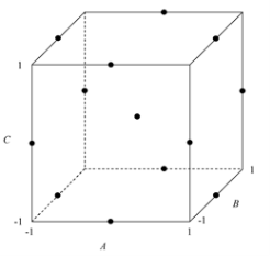
Figure 1.2 Schematic diagram representing the levels studied in a Box-Behnken Design
The number of experiments for Box-Behnken Designs can be calculated using Equation 1.7.
N= 2k (k-1) +C0
Where,
N= the number of experiments
k= the factor number
C0= the replicate number of the central point
For experiments in which there are three or less input variables the BBD design offers some advantage over the CCD approach, in that a fewer number of experimental runs are required. However this advantage does not exist when four or more parameters are to be investigated. A further advantage of BBD is that it does not include the need to evaluate situations in which all factors are simultaneously held at their highest and lowest levels. The use of a BBD therefore allows a formulation scientist to avoid undertaking experiments that are to performed under extreme conditions and that may produce substandard results due to the inclusion of data generated from these extreme high and low levels 37.
Doehlert Design
The Doehlert design is an experimental design approach in which different factors can be studied at different levels simultaneously43. This aspect of the Doehlert design is an important characteristic when using some input variables that may be subject to restrictions such as for example cost or experimental constraints (limited amounts of raw material or limited amount of time available) thereby making it a practical and economic alternative to other, second-order experimental design approaches37.This design describes a circular domain of two input variables, a spherical domain for three input variables and a hyper-spherical space for situations in which more than three input variables are to be investigated and which highlights the uniformity of the input variables to be studied in the experimental domain 37.
The schematic design space of a Doehlert design for two variables is shown in Figure 1.3, and is represented by a central point and six points of a regular hexagon.
An interesting feature of the Doehlert design is that new factors may be introduced during the course of a study without losing relevant and/or valuable information from the data already generated from the experimental runs that have already been completed.
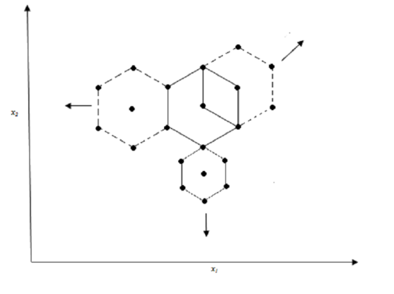 Figure 1.3 Schematic diagram representing the levels studied in a Doehlert Design
The number of experiments required for a Doehlert design is determined using Equation 1.8 37
N= k2+ k+ C0
Where,
N= the number of experiments
k= the factor number
C0= the replicate number of the central point
1.3.5 Mathematical Optimization
Optimization is a mathematical method used to determine an optimum response and is defined as the most advantageous state of existence of the system under investigation44. Multiple linear regression equations generated from statistically designed experiments provide a description of the change of a response with a change in input factors and further, allows for the determination of input variables that will produce an optimized response.
A difficulty that occurs in optimization procedures is the need to establish a compromise between the anticipated response variables. This challenge is often encountered in the process of optimization of tablets where the optimum tablet may be one that has superior strength and little or no friability, yet must also have a short disintegration time. Often an increase in tablet hardness results in an increase in the disintegration time of a tablet and therefore a compromise between these contradictory response variables is necessary to achieve an optimized formulation.
1.3.6 Advantages of RSM
The primary advantage of RSM in relation to classical experimental methods and approaches of data evaluation in which only one variable is investigated at a time, is that a large amount of information can be generated from a relatively small number of experiments 38. RSM is therefore less time and cost consuming than the classical approach that requires a large number of experiments to be conducted to be able to explain the behavior of a system 38, 39.
A further advantage, with the use of RSM is that it is possible to observe interaction effects of the independent input parameters on the response(s) being monitored 38. The model equation that is generated from the data is able to be used to explain the effect of combinations of independent input variables on the outcome of a process or product.
1.3.7 Disadvantages of RSM
A primary disadvantage of RSM is that fitting data to a second order polynomial for systems that contain some curvature is often not well accommodated by the second order polynomials that are produced. If the system cannot be explained by a first or second order polynomial, it may be necessary to reduce the range of independent input variables under consideration as this may then increase the accuracy of the model being considered38.
Another disadvantage is that although RSM has the potential to evaluate interaction effects of the independent input parameters, it is unable to be used to explain why an interaction(s) has occurred (210). A further disadvantage is that RSM is poor at predicting the potential outcomes for a system operated outside the range of study under consideration45
1.3.8 Software for Design of experiments
Many commercial software packages are available which are either dedicated to experimental design alone or are of a more general statistical type.
Software’s dedicated to experimental designs
DESIGN EXPERT
ECHIP
MULTI-SIMPLEX
NEMRODW
Software for general statistical nature
SAS
MINITAB
Cite This Work
To export a reference to this article please select a referencing stye below:
Related Services
View all


DMCA / Removal Request
If you are the original writer of this essay and no longer wish to have your work published on UKEssays.com then please click the following link to email our support team:
Request essay removal