Up-Gradient Particle Flux driven by Flow-to-Fluctuation

Up-Gradient Particle Flux driven by Nonlinear Flow-to-Fluctuation Energy Transfer in a cylindrical plasma device

• Lang Cui

Chapter 1

Introduction and Background

1.1 Fusion

1.1.1 Fusion reaction

Nuclear fusion is one of the most promising options for generating large amounts of carbon-free energy in the future. Fusion is the process that heats the Sun and all other stars, where atomic nuclei collide together and release energy. To get energy from fusion, gas from a combination of types of hydrogen – deuterium and tritium – is heated to very high temperatures (100 million degrees Celsius). Controlled fusion may be an attractive future energy options. There are several types of fusion reactions. Most involve the isotopes of hydrogen called deuterium and tritium [1]:

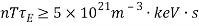
So far most promising method for fusion achievement is considered to through reaction by Eqn. (1.3) due to the fact that this reaction needs least energy and has largest nuclear cross section. As shown in Figure 1.1, every fusion reaction can provide 17.6 MeV nuclear energy of which 3.5 MeV is carried by α particles (helium nuclei) and the rest is carried by the neutron. Since both deuterium and tritium nuclei are carrying positive charges, we need to heat deuterium and tritium to a sufficiently high temperature (~ 10 keV) in order that thermal velocities of nuclei are high enough to overcome the Coulomb repulsion force to produce the fusion reaction. In fact, fusion reaction whether or not can be realized is given by the famous Lawson criterion [2]:

is the ion density, showing how good the particles are confined; is the energy confinement time, measuring the rate of the system loses energy to the environment. There also exists a minimum value of the energy confinement time defined as ratio of the total energy of the plasma to power loss []:

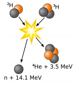
Figure 1‑1 the schematic of deuterium-tritium fusion reaction

1.1.2 Magnetic Confinement

There are two ways to achieve the temperatures and pressures necessary for hydrogen fusion to take place: Magnetic confinement uses magnetic and electric fields to heat and squeeze the hydrogen plasma. The most promising device for this is the ‘tokamak’, a Russian word for a ring-shaped magnetic chamber. The ITER project in France is using this method. Inertial confinement uses laser beams or ion beams to squeeze and heat the hydrogen plasma. Scientists are studying this experimental approach at the National Ignition Facility of Lawrence Livermore Laboratory in the United States.

Moreover, it is practically impossible to attain in the laboratory density levels near the ones in the star-centers. It is more feasible for controlled fusion purposes to work at low gas densities and increase the temperature to values considerably higher than that in the center of the sun. At these high temperatures all matter is in the plasma state, consists of a gas of charged particles that experience electromagnetic interactions and can be confined by a magnetic field of appropriate geometry. As shown in Figure 1.2, the motion of electrically charged particles is constrained by a magnetic field. When a uniform magnetic field is applied the charged particles will follow spiral paths encircling the magnetic lines of force. The motion of the particles across the magnetic field lines is restricted and so is the access to the walls of the container.[]

Figure 1‑2

When a single charged particle subject to a force is presented in an externally imposed magnetic field, the charged particle (ion/electron) will gyrate around the magnetic field lines. At the position of the guiding center, the charged particle will drift with a velocity which can be calculated from the fluid momentum equation, . The force can be due to an electric field ( drift), gravitational field, curvature drift ( drift) .etc. when there is a collection of charged particles, the force can also be a mean pressure gradient which can lead the particles to a diamagnetic drift with . The diamagnetic drift depends to the sign of the charge the particles carried, thus we expect to find a diamagnetic current in azimuthal direction and opposing the original magnetic field.

1.2 Drift wave turbulence and transport

1.2.1 Overview of Drift wave turbulence

It is known that drift waves result from the interaction between the dynamics perpendicular and parallel to the magnetic field due to the combined effects of spatial gradients, ion inertia, and electron parallel motion. Here “drift” refers to the diamagnetic drifts (perpendicular to both density gradient and magnetic field) due to dominant pressure gradient with a small finite and .

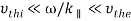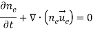
Derivation of drift wave dispersion relation can be found in many text books and review papers [1-3]. The experimental work performed in this dissertation was considered cool collisional plasma. An assumption is often made that , where is the drift wave frequency, and are the ion and electron thermal speed separately. Since drift waves have finite , electrons can move along magnetic field lines establishing a thermodynamic equilibrium among themselves. While the ion motions can be neglected. As a result, Landan damping is negligible. In absent of resonant particles, phase velocity distributions may reach to a fluid description of electrons and ions. We may apply the 2D fluid model to describe the system. Accounting for the fast gyromotion along magnetic field of the electrons for density and velocity , we have

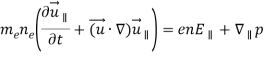
where is the electron pressure and denotes the direction parallel to magnetic field. By taking the limit and, a plane wave solution of the potential, 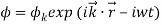we can then obtain the Boltzmann relation for electrons:

where and are the equilibrium electron density and temperature, . The schematics showing the physical mechanism of an electron drift wave can be seen in Figure 1.3. where the density perturbation is positive, the potential perturbation is positive. Similarly, where the density perturbation is negative, the potential perturbation is negative. The resulting electric field will cause a drift in the x direction. Since there is a gradient in the x direction, the drift will bring plasma of different density to a fixed point. Along with the quasi-neutrality condition, we can find the drift wave dispersion:

We notice that the drift waves travel with the electron diamagnetic drift velocity. Here the density and potential perturbations are in phase with a zero growth rate. Thus the plasma is stable.

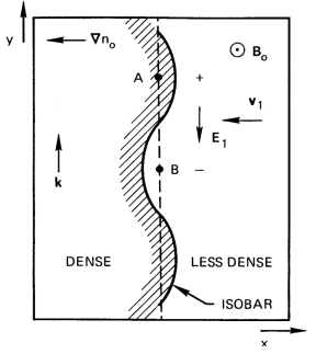
Figure 1‑3 Physical mechanism of a drift wave

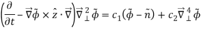
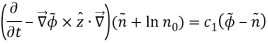
The fundamental property of electrostatic plasma turbulence is the drift wave frequency range in the absence of dissipation is often described by the Hasegawa-Mima Equations [4-6]. However, most experimental plasma condition is collisional like ours. Thus we are introducing a collisional drift-wave model described by Hasegawa-Wakatani equations, which derived from the same density continuity equation and electron momentum equation, but includes the electron parallel dissipation and the modifications of ion-neutral drag [4,7]. In a cylindrical geometry such as our machine, this model is written as two coupled dimensionless equations:

where = is the “adiabatic parameter” and is the normalized ion viscosity. We note here the density is normalized with , the potential with , time with , distance with , gyroradius. Here is the wavenumber parallel to magnetic field, is the electron collision frequency. Typically, the plasma is characterized by the ratio between the spatial scale of the collective modes () and the scale of the plasma (). HW model introduces the two main components to describe a weak drift wave turbulence system: linear instability driving mechanism and nonlinear damping for turbulence saturation.

For , parallel collisions are negligible thus the drift waves are linearly stable. Eqn. (1.11) and (1.12) will be reduced to the Hasegawa-Mima model:

For , this model goes to the hydrodynamic limit and reduces to the 2D Euler fluid equations.

Our experiments condition is satisfied with . In the presence of dissipation of the parallel electron motion (electrons can lose momentum to the background plasma as they move parallel to the magnetic field), the corresponding dissipation will cause a finite phase shift between density and potential fluctuations. As a result of the phase shift, the Boltzmann relation is no longer valid with :

Here the phase shift is the key for instability. The dispersion relation becomes:

where and . By solving for , we obtain

As we can see from Eqn. (1.16), the growth rate is always positive for a limited range of wavenumbers. This can be also understood from Fig. 1-3 that the phase shift causes drift velocity outwards where the plasma is already shifted outward. Hence the perturbation grows. The dissipation of parallel electron motion can occur via several different processes such as wave-particle interactions and electron-ion Coulomb collisions.

1.2.2 Particle transport

The energy losses observed in magnetic confinement devices are much greater than predicted by neoclassical transport theory and usually attributed to the presence of small-scale plasma turbulence. It is well known that spatial gradients in the plasma lead to collective modes called drift waves, which have wave numbers in the range of the observed density fluctuations. Drift waves in magnetized plasmas can produce various transports such as particle transport, momentum transport and kinetic energy transport. The magnetized plasma will convect around the maximum and minimum of density variations.

[1]F.F.Chen, Introduction to plasma physics and controlled fusion Second edition Volume 1: Plasma (Plenum Press, New York, 1984), second edn., Vol. 1.

[2]R. H. L. Hans R. Griem, Methods of Experimental Physics, Part A (Academic Press, New York and London, 1970).

[3]F. F. Chen, Phys Fluids 8, 1323 (1965).

[4]P. H. Diamond, A. Hasegawa, and K. Mima, Plasma Phys Contr F 53 (2011).

[5]K. Mima and A. Hasegawa, Phys Fluids 21, 81 (1978).

[6]Z. Yan, University of California, San Diego, 2008.

[7]N. A. Gondarenko and P. N. Guzdar, Geophys Res Lett 26, 3345 (1999).