Introduction to Atmospheric Modelling

• Yazdan M.Attaei

ABSTRACT

An atmospheric model is a computer program that produces meteorological information for future times at given locations and altitudes. Within any modern model is a set of equations, known as the primitive equations, used to predict the future state of the atmosphere [2]. These equations (along with the ideal gas law) are used to evolve the density, pressure, and potential temperature scalar fields and the air velocity (wind) vector field of the atmosphere through time. The equations used are nonlinear partial differential equations which are impossible to solve exactly through analytical methods, with the exception of a few idealized cases [3]. Therefore, numerical methods are used to obtain approximate solutions.

Get Help With Your Essay

If you need assistance with writing your essay, our professional essay writing service is here to help!
Find out more about our Essay Writing Service

In this work, we study the Heat and Wave equations as two important aspects when studying meteorology and atmospheric modeling. We assume an idealized domain with certain boundary conditions and initial values in order to predict the evolution of temperature and track the wave propagation in the atmosphere.

Keywords: Atmospheric model, Finite difference method, Heat equation, Wave equation.

Introduction:

An atmospheric model is a mathematical model constructed around the full set of primitive dynamical equations (equations for conservation of momentum, thermal energy and mass) which govern atmospheric motions. In general, nearly all forms of the primitive equations relate the five variables n, u, T, P, Q, and their evolution over space and time.

The atmosphere is a fluid. Therefore, modelling the atmosphere in fact means the numerical weather prediction which samples the state of the fluid at a given time and uses the equations of fluid dynamics and thermodynamics to estimate the state of the fluid at some time in the future.

The model can supplement these equations with parameterizations for diffusion, radiation, heat exchange and convection. The primitive equations are nonlinear and are impossible to solve for exact solutions and numerical methods obtain approximate solutions. Therefore, most atmospheric models are numerical meaning they discretize primitive equations. The horizontal domain of a model is either global, covering the entire Earth, or regional (limited-area), covering only part of the Earth [4]. Some of the model types make assumptions about the atmosphere which lengthens the time steps used and increases computational speed.

Global models often use spectral methods for the horizontal dimensions and finite-difference methods for the vertical dimension, while regional models usually use finite-difference methods in all three dimensions. Since the equations used are nonlinear partial differential equations, in order to solve them, boundary conditions and initial values are required. Boundary conditions are specified by the assumptions related to horizontal and vertical domain of study. The equations are initialized from the analysis data and rates of change are determined. These rates of change predict the state of the atmosphere a short time into the future; the time increment for this prediction is called a time step.

The equations are then applied to this new atmospheric state to find new rates of change, and these new rates of change predict the atmosphere at a yet further time step into the future. This time stepping is repeated until the solution reaches the desired forecast time. The length of the time step chosen within the model is related to the distance between the points on the computational grid, and is chosen to maintain numerical stability. Time steps for global models are on the order of tens of minutes, while time steps for regional models are between one and four minutes. The global models are run at varying times into the future.

Approximating the solution to the partial differential equations for atmospheric flows using numerical algorithms implemented on a computer has been intensively researched since the pioneering work of Prof. John von Neuman in the late 1940s and 1950s. Since Von-Neuman’s numerical experimentation on the first general purpose computer, the processing power of computers has increased at a breath-taking pace. While global models used for climate modeling a decade ago used horizontal grid spacing of order hundreds of kilometers, computing power now permits horizontal resolutions near the kilometer scale. Hence, the range of the scales of motion that next-generation global models will resolve spans from thousands of kilometers (planetary and synoptic scale) to the kilometer scale (meso-scale). Hence, the distinction between global climate models and global weather forecast models is starting to disappear due to the closing of the resolution gap that has historically existed between the two [1].

In this work first we solve two-dimensional heat equation numerically in order to study temperature rate of change which is a part of the equation for the conservation of energy in atmosphere. Two different types of sources (steady state and periodic pulse) are applied to simulate the heat sources for a local (small-scale) domain and the results are illustrated in order to investigate results for the applied boundary and initial value conditions.

In the second part of this study, two-dimensional wave equation is solved numerically using finite difference technique and certain boundary and initial value conditions are applied for the small-scale idealized domain. The aim is to study the wave propagation and dissipation along the domain from the results which are illustrated for different types of excitations (standing wave and travelling wave).

Overall, the aim of this paper is to show the efficiency of numerical solutions particularly finite difference method for solving primitive equations in atmospheric model.

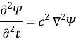
Heat Equation:

To study the distribution of heat in the domain, we consider following parabolic partial differential heat equation with thermal diffusivity a;

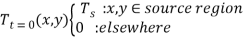
Domain: The idealized 2D domain is a plane of the size unity on each side with the following initial values and boundary conditions;

• Boundary Conditions (BCs): Dirichlet boundary condition is assumed for all the boundaries except at the regions where the source with T=T_s is taking place;

T (0,y)=0 , T(x,0)=0 (except at source)

T(1,y)=0 , T(x,1)=0

• Initial Values: At time zero, we assume temperature to be zero everywhere except at the region where the source is applied to;

Finite Difference Scheme: Heat equation can be discretized using forward Euler in time and 2^nd order central difference in space using Taylor series expansions and spatial 5-point stencil illustrated below;

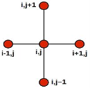
Figure 1: Five points stencil finite difference scheme

which after simplifying it takes the form;

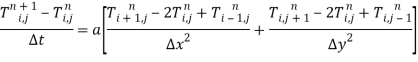
If we apply equal segmentation in both directions so that and rewriting the equation in the explicit form we have;

where .

For stability of our scheme we need hence;

Excitation: In order to observe the heat transportation in all directions, we assumed two different types of the source. First, we use a steady state source placed at the corner next to the origin with dimension of 5 grid cells with temperature amplitude T_s=10^o . The second source will be the following pulse source applied for 5 time steps and removed for the next 15 time steps (period of pulse function = 20). This will help to visualize the ability of the scheme to evaluate the temperature at the source region when the source is removed (back-transport of the heat).

Results: The following figures illustrate the results observed by applying the scheme, the sources described previously and thermal diffusivity of a=2 with grid cells of size (N_i=N_j=50 number of grid points in x and y directions);

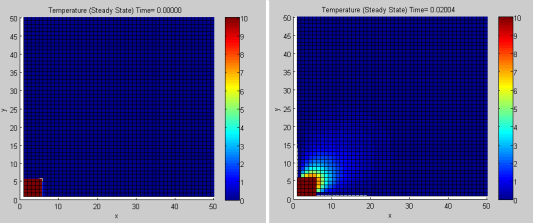
(a) (b)

Figure 2: Distribution of temperature (a) t=0 sec, b) t=20 msec, steady state source of size 5 grid cells in each direction.

It is observed that for t>0 while we have a constant temperature at the source, temperature is diffused along the domain in both directions and it will not diverge at any point when time increases since the stability criterion was already applied for the duration of time steps 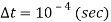. Also, in the vicinity of the source temperature is remained almost constant or with small variations after a sudden large increase due to the adjacent source cells with T_s=10^o and the nature of the scheme in which back grid points are included for approximation.

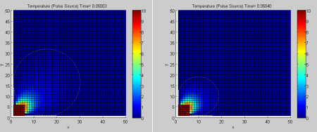
When the steady state source is replaced by a pulse source with certain On and Off duration (period) as it is seen in Figure 3, diffusion continues even in the absence of the source at the whole domain including the source region as in Figures 3(b),(d).

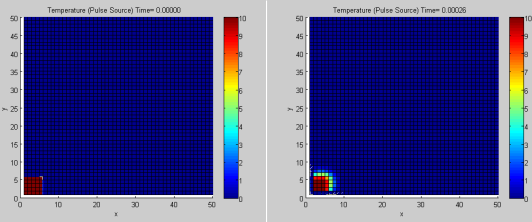
This is more visible in Figure 3(c) in the vicinity of the source but compared to the steady state excitation, there is a significant temperature drop due to the fact that the source has been Off for several time steps and temperature drops gradually with its maximum drop just before the source is applied again as illustrated in Figure 3(d).

(a) (b)

(c) (d)

Figure 3: Distribution of temperature when Pulse source is applied (period=20 time steps). (a)Initial time, (b)At first Off state, c)Right after second On state, d)Before 24^th On state

The last parameter to study for the heat equation is the diffusion coefficient. It is the coefficient which affects the rate of diffusion. Figure 4 shows that during equal time period, by larger coefficient heat will diffuse in larger area (dotted circles) of domain compared to when the coefficient is small.

(a) (b)

Figure 4: The effect of thermal diffusivity on temperature distribution.(a) a=2, (b) a=0.25

Wave Equation:

Similar to the heat equation, hyperbolic partial differential wave equation can be discretized by using Taylor series expansion. In this equation, c is the wave constant which identifies the propagation speed of the wave. Our goal is to study the reflection of the wave at the boundaries and the dissipation of the wave due to the numerical solution of the wave equation.

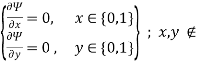
Domain: We use the same idealized domain in studying heat equation but in addition to Dirichlet, we also consider Von-Neumann boundary condition in order to study the reflection of the wave at the boundaries. A proper set of initial values will be chosen since this differential equation is of second order with respect to time.

• Von-Neuman Boundary Conditions: At the boundaries we will assume the following conditions;

Source region

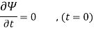
• Initial Conditions: The following initial conditions are assumed since we will use central difference in time and two time steps (current and previous) are used to evaluate the value at the future time;

)

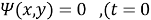Finite Difference Scheme: For the above parabolic differential wave equation, 2^nd order central difference scheme in both time and space is used for discretization as follows;

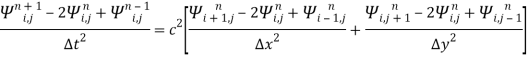
and with ∆x=∆y=h and rewriting the equation explicitly;

with

, the CFL number which must be less than or equal to since the coefficient of should be a positive (or zero) for stability of the scheme. Hence;

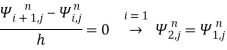
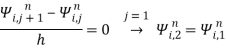
Now, back to the boundary condition, by using forward Euler difference for the left and bottom boundaries (i=1,j=1) we can write;

and similarly using backward difference at right and top boundaries (i=N_i,j=N_j) ;

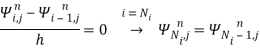
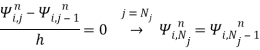
As we numerically solve for the derived general finite difference equation and illustrate it, we will see that the above boundary conditions are the mathematical representation of full wave reflection at the boundaries. For the second initial value condition we use central difference at t=0 (n=1) and it is derived;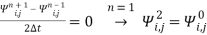

Substituting in general difference equation we get;

Now, we can apply second order central difference for both temporal and spatial variations for Von-Neumann boundary conditions.

Excitation: In this work, in order to study propagation and reflection of the wave using numerical solution of the wave equation, two different sources are applied at the origin with the dimension of 5×5 grid cells for both Dirichlet and Von-Neumann domain boundary conditions;

1. Travelling Wave:
2. Stationary Wave:

where 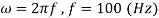and wave numbers 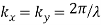. The wave constant c assumed to be c=1 for simplicity, therefore = 0.01 in both x and y direction.

Results: For Dirichlet boundary conditions the following figures are obtained for Stationary and Travelling wave sources;

1. (b)

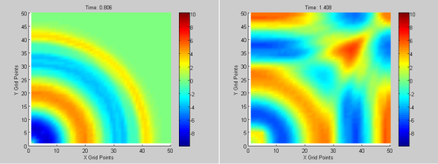
Figure 5: Dispersion of Stationary wave in domain with Dirichlet BCs (a) before reflection (b) after partial reflection

In Figure 5(a) the wave which is scattered from a stationary source is dissipated through the domain since the source is stationary. In Figure 5(b) the reflections at the boundaries are seen to be weak because of the Dirichlet BCs. Infact, these ripples are mostly due to the nature of finite differencing. However, it is clearly observed in Figure 6(a),(b) that the magnitude of the wave at the boundary is kept zero by Dirichlet BCs.

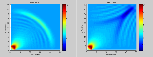
1. (b)

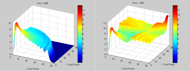
Figure 6: Dispersion of Stationary wave in domain with Dirichlet BCs (a) before reflection (b) after partial reflection, 3D view

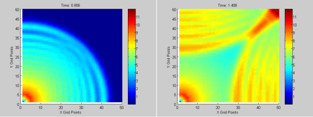
Figure 7 illustrates the travelling wave propagating in the domain. The ripples have larger magnitudes since the wave itself is travelling and this reduces the amount of attenuation because of the scheme specially after the reflection at the boundaries the weakend ripples are magnified by continuously incoming waves.

1. (b)

Figure 7: Travelling wave propagates in domain with Dirichlet BCs (a) before reflection (b) after partial reflection

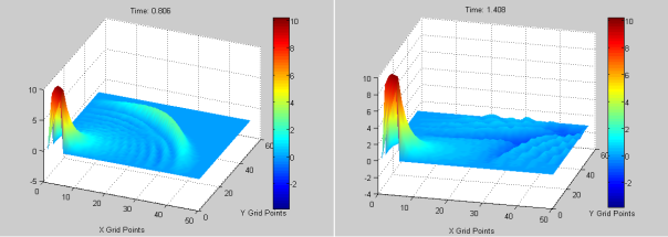
For Von-Neumann BCs, it is expected that for both standing wave and propagating wave we observe full reflection by the boundaries as described during the discretization of these BCs. Figures 8 and 9 illustrate the application of such boundary conditions for standing wave source and travelling wave source respectively.

1. (b)

Figure 8: Dispersion of Stationary wave in domain with Von-Neumann BCs (a) before reflection (b) after partial reflection

1. (b)

Figure 9: Wave propagation in the domain with Von-Neumann BCs (a) before reflection (b) after partial reflection

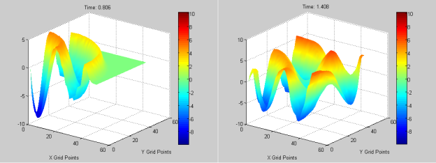
In the above figures, it is seen that at the boundaries the ripples are fully reflected back to the domain as well as the time when the wave is propagating forward from the source and is reflected at bottom and left boundaries. These would be more visible when showing the figures in three dimensions (Figure 10);

1. (b)

(c) (d)

Figure 10: Wave propagation (a),(b)standing wave, before and after reflection (c),(d)travelling wave, before and after reflection

To sum up, finite difference scheme which is used in this work provides numerical solution of the wave equation well and the results are close to what are expected for the wave propagation in such idealized domain with different boundary conditions.

Conclusion:

In atmospheric science, heat flow is related to temperature rate of change and the evolution of momentum and energy in atmospheric models are related the gravity waves as they transport energy. In the Earth’s atmosphere, gravity waves are a mechanism for the transfer of momentum from the troposphere to the stratosphere. Gravity waves are generated in the troposphere, propagate through the atmosphere without appreciable change in mean velocity. But as the waves reach more diluted air at higher altitudes, their amplitude increases, and nonlinear effects cause the waves to break, transferring their momentum to the mean flow.

Therefore, numerical solutions of atmosphere primitive equations play an important role for studying the evolution of fundamental variables in atmospheric science especially since these equations are partial differential equations which cannot be solved analytically.

In this paper, a brief study over the numerical solution of heat and wave equations was conducted as a basis for a bigger scale atmospheric modelling. The results demonstrate the efficiency of finite difference method to solve these equations (in small-scale domain) when they are compared to the theoretical expectations, therefore, solving primitive equations in atmospheric models by numerical techniques can be a following work to this paper.

REFERENCES