Finding 'G' Using Simple Pendulum Experiment

Abstract

This report shows how to find an approximate of ‘g’ using the simple pendulum experiment. There are many variables we could see into, some of them are displacement, angle, damping, mass of the bob and more. However the most interesting variable is, the length of the swinging pendulum.

Get Help With Your Essay

If you need assistance with writing your essay, our professional essay writing service is here to help!
Find out more about our Essay Writing Service

The relationship between the length and the time for one swing (the period) has been researched for many years, and has allowed the famous physicists like Isaac Newton and Galileo Galilei to get an accurate value for the gravitational acceleration ‘g’. In this report, we will replicate their experiment, and will find an accurate value for ‘g’. Finally it will be compared with the commonly accepted value of 9.806 m/s² .

Introduction

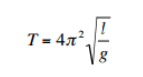
A simple pendulum performs simple harmonic motion, i.e its periodic motion is defined by an acceleration that is proportional to its displacement and directed towards the Centre of motion. Equation 1 shows that the period T of the swinging pendulum is proportional to the square root of the length l of the pendulum:

With T the period in seconds, l the length in metres and g the gravitational acceleration in m/s². Our raw data should give us a square-root relationship between the period and the length. Furthermore, to find an accurate value for ‘g’, we will also graph T² versus the length (l) of the pendulum. This way, we will be able to obtain a straight-line graph, with a gradient equal to 4π2g^-1 .

Equipment and Method

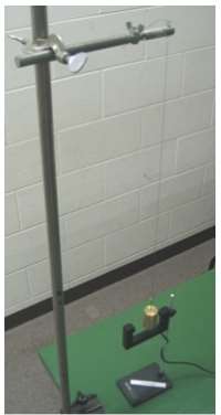
For this investigation, limited resources like, clamps, stands, a metre ruler, a stopwatch, a metal ball (bob), and some string were used. The experimental set-up was equal to the diagram, shown in figure 1.

In this investigation, the length of the pendulum was varied (our independent variable) to observe a change in the period (our dependent variable). In order to reduce possible random errors in the time measurements, we repeated the measurement of the period three times for each of the ten lengths. We also measured the time for ten successive swings to further reduce the errors. The length of our original pendulum was set at 100 cm and for each of the following measurements, we reduced the length by 10 cm.

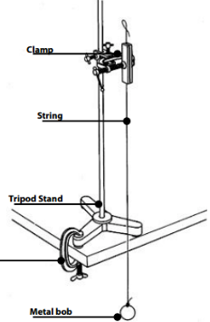
Figure 1

As stated earlier, it was decided to measure the time for ten complete swings, in order to reduce the random errors.

These measurements would be repeated two more times, and in total ten successive lengths were used, starting from one metre, and decreasing by 10 cm for each following measurement.

A metre ruler was used to determine the length of the string. One added difficulty in determining the length of the pendulum was the relative big uncertainty in finding the exact length, since the metal bob added less than a centimeter to our string length, measured from the bob’s centre. This resulted in an uncertainty in length that was higher than one would normally expect. The table clamp was used to secure the position of the tripod stand, while the pendulum was swinging.

After the required measurements, one experiment was carried out to find the degree of damping in our set-up. Damping always occurs when there is friction, but exactly how significant the degree of damping in our experimental set-up was, remained uncertain.

Depending on the degree of damping, it may or may not have a significant effect on our measurements.

All measurements were taken under the same conditions, using the same metal bob, the same ruler, in the same room, and at approximately 26 degrees Celsius.

Data Collected

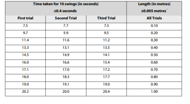
Table 1

In table 1 the ±o.46 sec uncertainty in time was obtained by comparing the spread for the different measurements. The time measurement for the 0.50 metre length, had the largest spread (±0.4 seconds), and was therefore used as the uncertainty in the time measurement.

In table 1 the theoretical uncertainty in the length measurement would be 0.05 cm (a metre ruler was used). However, in the experimental set-up, the two end points (the one tied to the clamp, and the one tied to the metal bob) gave rise to a bigger uncertainty, as the exact end-points could not be precisely determined. We estimated the uncertainty in length to be 0.5 cm, or 0.005 metres.

These data in table 1 need to be processed, before we can continue our analysis. First of all, the average of the three trials need to be found, which will reduce our error. Secondly, the time for one swing (or one period) must be found, which will reduce our absolute error, but not our percentage error.

It should also be noted, that for all the measurements, a constant, and small, angle of maximum displacement (amplitude) was used. The angle was kept between 5° to 7°, small enough to ignore the friction present in our experimental set-up.

Apart from these measurements, one more experiment was done to see how much damping was present in our set-up. It took, on average, between 100 and 150 swings, before the motion had seemed to stop. This showed that there was damping present, but this did not significantly affect the measurement of just ten swings.

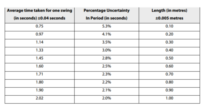
Table 2 shows the processed data and the uncertainties.

While drawing the graph for the data in table 2, the relationship between the variables used is clearly not a linear one. The suggested square-root relationship shows it, and to linearise this curve, it must be interchanged and the axis must be modified. (the graph is shown in Graph 1)

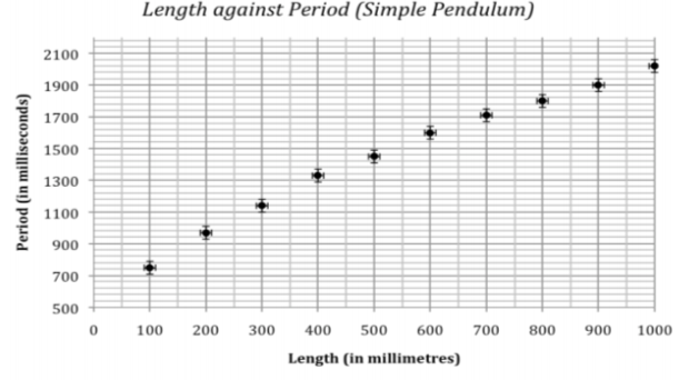
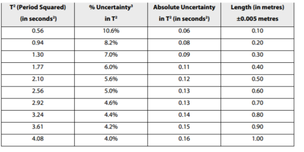
Table 3

Based on the theory of Simple Harmonic Motion and equation 1, it should be a linear relationship between T² and Length. When graphing these two modified variables, the regression line must be linear, passing through point (0,0) and with a gradient equal, or close to 4π2g^-1 .

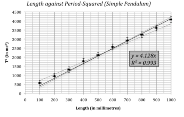
Graph 2

Conclusion and Evaluation

Graphing the length against T² clearly shows a linear relationship, in agreement with the theory. The actual line of best fit does not go through (0,0) which suggests a systematic error in our experiment. But when graphing a line of best fit, with the condition it should pass through (0,0), we find a line with a gradient of 4.128 and a correlation coefficient of 0.993, which further suggests a very strong linear correlation between our chosen variables.

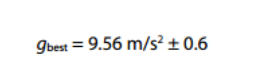
The value for ‘g’ can be calculated by dividing 4π² with the gradient of the line of best fit;

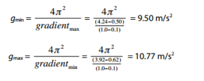
The uncertainty in this value was found, by taking half the difference of the lowest possible value for ‘g’ and the highest possible value for ‘g’:

Comparing our calculated value for the gravitational acceleration ‘g’ with the accepted theoretical value gives us an error of 2.5%, well within the error margins that we calculated. This is a reasonable result, given the equipment and the time constraints that we faced.

Looking at our graph, we cannot identify any outliers. However, our data values suggest a line of best fit that does not pass through (0,0). When we do fit a linear regression onto our data values, that passes (0,0), we see that the line does not ‘hit’ all the horizontal error bars (the uncertainty in the length). This may suggest a systematic error in the measurement of the length of our pendulum.

Further Improvements

To reduce the systematic error in the length measurements, one should take accurate measurements of the diameter of the metal bob used. In this experiment, it looks as if we systematically used a length for the pendulum that was too short. If 1 cm was added to our data, we would get a value for ‘g’ that is equal to the theoretical value of 9.806 m/s² .

The theoretical value used, is the average value for ‘g’ on Earth, and may be slightly different from the one that was measured.

Instead of three measurements, taking five measurements would be better, as it would not take too much extra time, and this would further reduce our uncertainty in the measurement of the period of swing.

Alternatively, measuring the time for 20 swings, instead of 10 swings, would also reduce the uncertainty in time.

Lastly, a photogate could be used in the future, to measure the period with higher precision. A nice extension to this experiment would be the use of different metal bobs, of different diameter and/or mass. This would allow us to calculate the effect of air resistance on this experiment.

References

1. http://physics.nist.gov/cgi-bin/cuu/Value?gn
2. http://www.practicalphysics.org/go/Experiment_480.html
3. http://en.wikipedia.org/wiki/Simple_harmonic_motion#Mass_on_a_spring
4. http://www.phys.utk.edu/labs/simplependulum.pdf