Density Functional Theory (DFT): Literature Review
| ✅ Paper Type: Free Essay | ✅ Subject: Physics |
| ✅ Wordcount: 2542 words | ✅ Published: 01 Feb 2018 |
Theoretical Background and Literature Review
2.1 Density Functional Theory
This section covers basics about Density Functional Theory (DFT), which is the theoretical method behind our investigations. For those who are interested in a much more deep knowledge about the DFT we refer to textbooks such as [29] and [30].
2.1.1 History of Density Functional Theory
To get precise and accurate results from both theoretical and computational methods, the scale of physical phenomena must be well defined. In physics and material science the relevant scales of matter are time and size. In computational material science, for the multiscale understanding in both time and size scale the smallest relevant scale of atomic interactions are best described by ab initio techniques. These techniques are based on the determination of electronic structure of the considered materials and an intelligent transfer of its characteristics to higher-order scales using multidisciplinary schemes. More specifically, if the interaction of electrons is solely described using universal principles such as the fundamental laws of quantum mechanics condensed in the Schrodinger equation, these simulations are called firstprinciples, or ab initio methods. One can also separate those methods as Hartree-Fock and post-HF techniques that mainly uses by quantum chemistry field and Density Functional Theory (DFT) which is typically used in of material science.
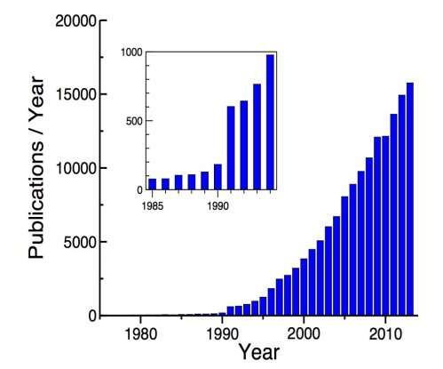
Ab initio simulations are becoming remarkably popular in scientific research fields. For example in DFT case, in a simple search at Web Of Science
[31] or any other publication search tool, one can easily see that number of publications that include ”Density Functional Theory” in their title or abstract is over 15000 in 2013. Therefore, it can be concluded that, ab initio based research already an important third discipline that makes the connection between experimental approaches and theoretical knowledge.
Figure 2.1: Usage trend of DFT over years
Within ab initio simulations quantum mechanical equations for any system that may be ordered or disordered are solved. That actually gives one drawback which is, solving that kind of equations is generally only possible for simple systems, because of the expensive electron-electron interaction term. So, in general, the ab initio simulations are restricted to 150-200 atoms calculations with most powerful computer clusters. Due to the that severe limitation, better techniques and methods are developed and implemented to bring the real materials into realm of ab initio simulations. The major development of ab initio methods with practical applications took place when many electron interactions in a system was possible to be approximated using a set of one electron equations (Hartree-Fock method) or using density functional theory
In 1927, Thomas [32] and Fermi [33] introduce a statistical model to compute the energy of atoms by approximate the distribution of electrons in an atom. Their concept was quite similar to modern DFT but less rigorous because of the crucial manybody electronic interaction was not taken into account. The idea of the Thomas and Fermi was that, at the starting point for simplicity that electrons do not interact with each other and using classic terms, therefore, one can describe the kinetic energy as a functional of electron density of non-interacting electrons in a homogeneous electron gas. 3 years later, in 1930, Dirac [34] succeeded to include the many-body exchange and correlation terms of the electrons and actually he formulated the local density approximation (LDA), that is still used in our days. However, the Thomas-Fermi and Dirac model that are based on homogeneous electron gas do not cover the accuracy demand in current applications.
In same the years as Thomas and Fermi, Hartree [35] also introduce a procedure to calculate approximate wavefunctions and energies for atoms and that was called Hartree function. Some years later, to deal with antisymmetry of the electron system, his students Fock [36] and Slater[37], separately published self-consistent functions taking into account Pauli exclusion principals and they expressed the multi-electron wavefunction in the form of single-particle orbitals namely Slater-determinants. Since the calculations within the Hartree-Fock model are complicated it was not popular until 1950s.
The fundamental concepts of density functional theory were proposed by Hohenberg and Kohn in their very well known paper in the year 1964 [38]. The main idea was trying to use the electron density instead of complex and complicated wavefunction. A wavefunction contains 3N variables, where N is the number of electrons and each electron has 3 spatial degrees of freedom. In contrast to that electron density contains only 3 variables. Therefore, the implementation of the electron density with 3 variables will be more easy to handle than 3N wavefunction variables. In their work, Hohenberg and Kohn proved that all ground state properties of a quantum system, in particular the ground state total energy, are unique functionals of the ground state density. However, the Hohenberg-Kohn (HK) formulation is not useful for
actual calculations of ground state properties with enough accuracy.
A major improvement was achieved one year later, in 1965. Kohn and Sham [39] proposed a formulation by partially going back to a wavefunction description in terms of orbitals of independent quasi particles. The main idea was that the many-body problem can be mapped onto a system of non-interacting quasiparticles. This approach simplified the multi-electron problem into a problem of non-interacting electrons in an effective potential. This potential includes the external potential and the effects of the Coulomb interactions between the electrons, e.g., the exchange and correlation interactions. Since then up to now the Kohn-Sham equations are used in practically all calculations based on DFT.
2.1.2 Schr¨odinger’s Equation
In quantum mechanics, analogue to Newtons equations in classical mechanics, the Schr¨odinger equation is used. This is a partial differential equation and used to describe the physical quantities at the quantum level. The Schr¨odinger equation forms the basis of many ab initio approaches and its non-relativistic form is an eigenvalue equation of the form:
HˆΨ(ri,Rj)= EΨ(ri,Rj) (2.1)
where Ψ(ri,Rj) is the wavefunction of the system depending on the electron coordinates ri,i =1…N and the coordinates of all nuclei in the system Rj,j =1…M. Hˆis the Hamiltonian of a system that contains M nuclei and N electrons. Therefore, the Schr¨odinger equation that involves both nuclei and electrons has to be solved for the many-body eigenfunctions Ψ(r1,r2, …, rN ; R1,R2, …, RM ). The many-body Hamiltonian can be written in the form:
Hˆ= Tˆe + Tˆn + Vˆnn + Vˆen + Vˆee (2.2)
ˆˆ
where all of parts are operators. Te and Tn are the kinetic energies of the ˆˆ
electrons and nuclei, respectively. Ven, Vee and Vˆnn represent the attractive electrostatic interaction between the electron and the nuclei and the repulsive potential due to the electron-electron and nucleus-nucleus interactions.
One can also write them down explicitly:
N
f2
ˆ
Te = −
2
i
(2.3)
2me
i=1
M
2Mn
n=1
f2
ˆ
Tn = −
2
n
(2.4)
11
M
ZnZme2
= (2.5)
4π 0 2 |Rn − Rm|
=1;n,mn
=m
ˆ
Vnn
ˆ
Ven = −
11
MN
Zne2
(2.6)
4π 0 2 |ri − Rn|
n=1 i=1
j=
M
e
= (2.7)
4π 0 2 |ri − rj|
i,j=1;i
2
11
ˆ
Vee
where me and Mn are the electron and nuclei masses, Zn is the nuclear number of the n-th atom, e is the electronic charge and f is the Planck constant. For simplicity one can also use atomic units. Then the Hamiltonian takes the form:
NMM
ZnZm
in
22 |Rn − Rm|
i=1 n=1 n,m=1;n
=m
1
1
ˆ
H = − 2 2
−
+
(2.8)
j=
MNMZn
− +
|ri − Rn||ri − rj|
n=1 i=1 i,j=1;i
2.1.3 Born-Oppenheimer Approximation
It is clear that forces on both electrons or nuclei is in the same order of magnitude because of their electric charge. Therefore, the expected momen
1
tum changes due to that forces must be the same. However electrons are much smaller than nuclei (e.g. even for Hydorgen case nuclei nearly 1500 times larger than an electron) they must have higher velocity than nuclei. One can conclude that electrons will very rapidly adjust themselves to reach the ground state configuration if the nuclei start moving. Born and Oppenheimer [40] published their work in 1927, they simply separated the nuclear motion from electronic motion which is now known as the Born-Oppenheimer approximation. Therefore, while solving the Hamiltonian Equation in (2.8) one can simply assume nuclei as stationary and solve the electronic ground state at first then calculate the energy of the system in that configuration and solve the nuclei motion. Then the separation of electronic and nuclear motion leads to an separation of the wavefunctions Ψ = ψφ of electrons and nuclei, respectively. Via the separation one can treat the nuclear motion externally by not including the Hamiltonian and the “electronic” Hamiltonian can be written as:
Hˆe = Tˆe + Vˆen + Vˆee (2.9)
Solving the equation (2.9), one can get the total energy of the ground state of the system, which can be defined as:
E0 = ψ0|He|ψ0 + Vnn (2.10)
where E0 is the ground state total energy of the system and ψ0 is the eigenfunction of the electronic ground state.
2.1.4 Hohenberg-Kohn Theorem
However, the Hamiltonian in Equation (2.9) is quite complicated to solve for realistic systems due to the high number of electrons and especially the term Vee makes it impossible to solve the problem exactly. Therefore, instead of solving the many-body wavefunctions, Hohenberg-Kohn deal with that problem by reducing it to the electron density ρ(r). This approach makes the fundamentals of DFT. According to Hohenberg and Kohn, the total energy of the system can be defined via the electron density as E = E[ρ(r)] and it will be the minimum for the ground state electron distribution, namely ρ0(r). Therefore, the exact theory of many-body systems reduced to the electron density that can be defined as:
ρ(r)= … d3 r2…d3 rN |ψ(r1, …rN )|2 (2.11)
and has to obey the relation:
ρ(r)d3 r = N (2.12)
where N is the total number of electrons in the system. One can also summarize the HK theorem in the form of the two main theorems,
- Theorem I : The external potential vext(r), which is the potential energy generated by the nuclei, can be determine from the ground state electron density ρ0(r). Then Hamiltonian will be fully defined, also the wavefunction for the ground state will also be known.
- Theorem II : E0,the ground state total energy of the system with a particular vext will be the global minimum when ρ = ρ0.
From the perspective of these two theorems one can write down the total electronic energy as:
E[ρ]= Te[ρ(r)] + ρ(r)vext[ρ(r)] + EH [ρ(r)] + Exc[ρ(r)]d3 r (2.13)
One can also add the kinetic energy of the electrons T − e[ρ(r)], the classical Coulomb interaction (or Hartree interaction) between electrons EH [ρ(r)] and the remaining complex non-classical electron exchange correlations Exc[ρ(r)] into an universal functional FHK [ρ(r)]:
E[ρ]= FHK [ρ]+ ρ(r)vext[ρ(r)]d3 r (2.14)
The remaining will be to apply the variational principle to extract the ground state energy
δE[ρ(r)]
|ρ=ρ0 = 0 (2.15)
δρ(r)
2.2 Kohn-Sham Equations
However, the Equation (2.14) does not give an accurate solution. In that point, Kohn and Sham reformulated the current approach and introduced a new scheme by considering the orbitals by mapping the fully interacting electronic system onto a fictitious system of non-interacting quasi particles moving in an effective potential.The Kohn-Sham equations solution can be written as:
ˆ
HKSψi = iψi (2.16) where the Hamiltonian is
HˆKS =[− 1 2 + Veff (r)] (2.17)
2
Therefore, the problem of finding the many-body Schr¨odinger equation is now replaced by solving single particle equations. Since the KS Hamiltonian is a functional of just one electron at the point r then the electron density can be defined according to HK theorem:
occ.
ρ(r)= |ψi(r)|2 (2.18)
i=1
Besides, kinetic energy term and the classical Coulomb interaction energy of the electrons can be define as:
N
1
d3
Te = − r|ψi(r)|2 (2.19)
2
i=1
1 ρ(r)ρ(r )
EH [ρ]= d3rd3 r(2.20)
2 |r − r | Then the Hohenberg-Kohn ground state energy cn be written according to Kohn-Sham approach:
N
δExc
EKS = i − EH [ρ]+ Exc − (2.21)
δρ(r)
i
i are the one electron energies and are coming from the results of KS equations results, however it has low physical meaning. The most significant term in the Equation (2.20) is the last term. which is the exchange correlation term that contains all the many-body interactions of exchange and interactions of the electrons. One can also write down it as in the form of Hohenberg-Kohn universal functional from the equation:
Exc[ρ]= FHK [ρ] − (Te[ρ]+ EH [ρ]) (2.22)
The total ground state energy can be obtained from EKS in Equation (2.21). Since it contains only the electronic energy, the total ground state energy of the system is calculated by adding the nuclei-nuclei repulsion term:
E0(R1, …, RM )= i − EH [ρ0]+ Exc[ρ0] − vxcρ0dr + Vnn(R1, …, RM )
(2.23) where E0 is the total ground state energy for a given atomic configuration (R1, …, R2). Therefore, the total energy depend on ionic positions that is actually depends on the volume and cell shape, so one can easily compute the ground state structure by minimizing the total energy. Also one can find the force acting on the particular atom, say atom A, by taking the derivative of the energy with respect to ionic position of A:
δE0(R1, .., RM )
FA(RA) = (2.24)
δRA
which also shows the total energy dependence on atomic positions.
2.3 Calculating the Exchange-Correlation Energy
The derived and briefly explained KS equations from the fundamentals of all modern DFT calculations today. The most important point in the solution of KS equations are the exchange-correlation functional Exc which also determines the quality of the calculation. There are two well known approximation methods to get the exchange correlations: local density approximation (LDA)[39] and generalized gradient approximation (GGA)[41, 42].
2.3.1 Local Density Approximation
The local density approximation starts with a very simple approximation that, for regions of material where the charge density is slowly varying, the exchange-correlation energy at that point can be considered as the same as for a local uniform electron gas of the same charge density. In that case one can write the Exc as:
Exc = ρ(r) xc(r) (2.25)
where xc(r) is the exchange correlation energy per electron in an homogenous electron gas of density ρ(r). Even though the approximation is seemingly simple it is suprisingly accurate. However, it also has some drawbacks such as under-predict on of ground state energies and ionisation, while overpredicting binding energies as well as slightly favouring the high spin state structures and does not work fine for some systems where the charge density is rapidly changing.
2.3.2 Generalized Gradient Approximation
Knowing the drawbacks of LDA the most logical step to go beyond LDA is not to limit oneself to the information about the charge densitiy ρ(r) at a particular point r, but also adding the information about the gradient of the charge density ρ(r) to be able to take into account the unhomogeneous density in the system. Then one can write the exchange correlation energy as :
Exc[ρ]= f(ρ, ρ)dr (2.26)
That way of description leads to an improvement over LDA, nevertheless in some systems LDA still works better. There also several different parameterizations of GGA while in LDA its only one. In GGA some of these parameterizations are semi-emprical, in that experimental data (e.g. atomization energies) is used in their derivation. Others are found entirely from first principles. A commonly used functional is the PW91 functional, due to Perdew and Yang [43, 44] and most commonly used today is PBE [45, 46] by Perdew, Burke and Ernzerhof.
2.4 Ultra-Soft Pseudopotentials and the Projector-Augmented Wave Method
In the previous section, the calculation of Exc is described. Nevertheless this is not the single sensitive point of DFT calculations. The other point is the treatment of the electron-nuclei interaction. There are several available methods that describes the electron-nuclei interaction, but the most effective
Cite This Work
To export a reference to this article please select a referencing stye below:
Related Services
View all


DMCA / Removal Request
If you are the original writer of this essay and no longer wish to have your work published on UKEssays.com then please click the following link to email our support team:
Request essay removal