Power Flow Studies Using MATLAB
| ✅ Paper Type: Free Essay | ✅ Subject: Mathematics |
| ✅ Wordcount: 2700 words | ✅ Published: 23 Sep 2019 |
Power Flow Studies Using MATLAB
Executive Summary
The report aims to show the differences between Newton-Raphson and Gauss-Seidel methods by using them to analyse a power flow system. During the study in a two-bus system, with a slack bus and PQ bus, two convergence tolerances were used. The case study 1 compares the iterative process of the two methods for a voltage tolerance convergence and case study 2 compares the iterative process of the two methods for a power mismatch convergence. The main points that investigated are the results and the speed of convergence. Although, both methods converge to the same values, Newton-Raphson converges exponentially and compared to Gauss-Seidel which converges linearly, needs only around half iterations to return the expected result.
Table of Contents
Power Flow Study Results and Analysis
Introduction
A load or power flow analysis is a computational procedure required to determine the sinusoidal steady state of the entire power system. The mathematical solution includes a system of nonlinear algebraic equations, which during an iterative process, the values converge to only one solution. The outcome of the power flow analysis is the acquisition of the voltage magnitudes and angles at each bus. Once the voltage magnitudes and angles at each bus have been acquired using power flow analysis, the real and reactive power at each branch of the power system can be computed. Furthermore, losses in particular lines can be computed by investigating the difference between the power flow in the sending and receiving ends and by determining over and under load conditions, the appropriate solution is taken into consideration. In the power industry, load flow analysis is used on a daily basis as it is essential in determining the fault-free, stable and economical operation of existing power systems, as well as for future expansion of power systems.
A two-bus system is given in Figure 1 below.
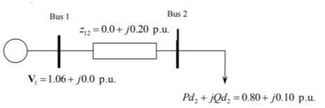
Figure 1: Two-bus System
The power system consists of a slack bus, which is illustrated as bus 1 and a load bus, which is illustrated as bus 2.
Bus 1 is a slack bus (or swing, or reference) and its main role is to be the phase angle reference of the system. It also balances the active power |P| and reactive power |Q| in a system by injection in circumstances when is required. It is a reference bus for which the voltage magnitude and angle are input data
and the active power |P| and reactive power |Q| are the unknown quantities need to be calculated by the power flow analysis. Usually the
is
, however in this assignment should be considered as
.
Bus 2 is a load (P-Q) bus which absorbs power from the system. The active power |P| and reactive power |Q| are quantified and voltage magnitude |V| and angle |δ| need to be computed.
Background Theory
Newton-Raphson Method
The Newton-Raphson method is a powerful method for maximising an objective function by using quadratic convergence of approximations [1].
A number of nonlinear algebraic equations is given in matrix format
where x and y are N vectors and
is an N vector of functions. The aim is to solve for x, accounting that
and y are given. By rewriting eq. 1.1
Then, by adding Dx to both of the eq. 1.2
, where D is a square NxN invertible matrix. Then, multiplying by
in both parts
The values of x on the left side are used to calculate the next values of x on the right side, so that
For non-linear equations, it is necessary that matrix D must be specified. One of the methods of specifying matrix D called the Newton-Raphson method.
The Newton-Raphson method is based on the Taylor series expansion of
.
By neglecting the higher order terms in eq 1.6
During the Newton Raphson iteration process,
is been replaced by the old value x and x by the new value
To continue to the next step, the
Jacobian matrix is used.
where the elements inside the Jacobian matrix are partial derivatives. Therefore, by substituting the Jacobian matrix into eq. 1.7.
(1.9)
Instead of computing the inverse of the Jacobian matrix
, it can be rewritten as :
, where
The Newton-Raphson method converges to the result in each iteration and depending on the convergence tolerance we can select the precision needed. The steps below show the process during each iteration.
Step 1 By using the eq. 1.12, we compute
Step 2 By using the eq. 1.8, we compute
Step 3 By using Gauss elimination and back substitution, we solve the eq. 1.10 in order to find
Step 4 Finally we compute
from eq. 1.11. Compare
with
to find the convergence tolerance to determine the precision of the result. [2]
Power Mismatch
The equation for complex power expressed as
:
From equation 1.13, the current injection into any bus I can be expressed as:
where,
terms are admittance matrix elements. Then, we substitute eq. 1.14 into eq. 1.13:
where, Vk is a phasor, with magnitude and angle
. Moreover, the admittance matrix is complex with real and imaginary parts
. Then, by rewriting eq. X as
A phasor may be also expressed as a function of sinusoids
Then by rewriting the eq. 1.19 we get:
Then by performing the multiplications inside the parenthesis and by splitting the equation into real and imaginary parts, we can find the active (
) and reactive (
) power.
These two equations called the power flow equations and are used as fundamental equations for load flow analysis.
Jacobian matrix for a two-bus power system:
Gauss-Seidel Method
The Gauss-Seidel method used as an iterative process to solve a square system of linear equations. It uses the form
To do a power flow analysis into a power system, a set of linear equations
analogous to y=Ax needs to be solved. For every load bus load bus,
can be calculated from
The Gauss-Seidel method equation is
By using eq. 2.3 and applying it to the nodal equations
Power Flow Study Results and Analysis
Case Study 1
This case study will focus on the comparison of the Newton-Raphson and Gauss-Seidel methods by drawing a relationship
vs number of iterations using a voltage convergence tolerance of
.
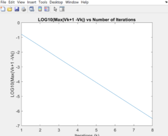
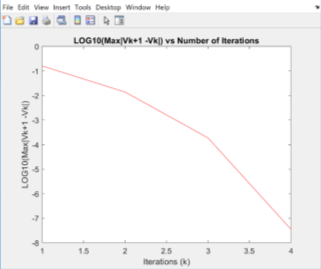
Figure 2: Newton-Raphson method with voltage convergence tolerance
Figure 3: Gauss-Seidel method with voltage convergence tolerance
|
|
||
|
Iterations(k) |
Newton-Raphson Convergence |
Gauss-Seidel Convergence |
|
1 |
-7.96567e-01 |
-7.82716e-01 |
|
2 |
-1.85971e+00 |
-1.59734e+00 |
|
3 |
-3.72734e+00 |
-2.42426e+00 |
|
4 |
-7.45094e+00 |
-3.24175e+00 |
|
5 |
-4.05939e+00 |
|
|
6 |
-4.87682e+00 |
|
|
7 |
-5.69426e+00 |
|
|
8 |
-6.51169e+00 |
Table 1: Comparison of Newton-Raphson and Gauss-Seidel solutions with voltage convergence tolerance
|
Newton-Raphson |
Gauss-Seidel |
|
|
Active Power Injection at Bus 2 |
8.00000e-01 |
8.00000e-01 |
|
Reactive Power Injection at Bus 2 |
2.22751e-01 |
2.22752e-01 |
|
Voltage Magnitude at Bus 2 |
1.02910e+00 |
1.02910e+00 |
|
Voltage Angle at Bus 2 (rad) |
-1.47206e-01 |
-1.472059e-01 |
Table 2: Comparison of the Active and Reactive Power Injection values and the Voltage magnitude and angle values between the Newton-Raphson and Gauss-Seidel solutions
The two graphs above show the voltage convergence of the voltage at bus 2 using Newton Raphson and Gauss-Seidel method respectively. For the Gauss-Seidel solution, it takes eight iterations till the value of the change between each iteration (
) is below the voltage convergence tolerance (
). From the other side, Newton-Raphson method converges in half iterations, showing the quadratic convergence of the method, in contrast with the Gauss-Seidel method, which converges linearly. The difference between the two methods can be shown in table 1, as the difference between each iteration for the Gauss-Seidel method is the same, comparatively with the Newton-Raphson which the difference doubles in each iteration. Furthermore, at the beginning both methods have the same gradient, but Newton-Raphson’s gradient sharply converges closer to the result. Finally, there is no difference in active and reactive power and voltage magnitude and angle calculated by both methods. This could be due to restriction of decimal places and little changes would exist if we had more decimal places.
Case Study 2
This case study will focus on the comparison of the Newton-Raphson and Gauss-Seidel methods by drawing a relationship
vs number of iterations using a power convergence mismatch of
.
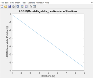
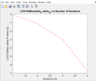
Figure 4: Newton-Raphson method with power mismatch tolerance
Figure 5: Gauss-Seidel method with power mismatch tolerance
|
LOG10(Max |deltaP -deltaQ|) |
||
|
Iterations(k) |
Newton-Raphson Convergence |
Gauss-Seidel Convergence |
|
1 |
-9.69100e-02 |
-9.69100e-02 |
|
2 |
-1.14339e+00 |
-9.06578e-01 |
|
3 |
-3.01934e+00 |
-1.72616e+00 |
|
4 |
-6.75115e+00 |
-2.56041e+00 |
|
5 |
-3.36113e+00 |
|
|
6 |
-4.19571e+00 |
|
|
7 |
-4.99599e+00 |
|
|
8 |
-5.83058e+00 |
|
|
9 Table 3: Comparison of Newton-Raphson and Gauss-Seidel solutions with power mismatch tolerance |
-6.63085e+00 |
|
Newton-Raphson |
Gauss-Seidel |
|
|
Active Power Injection at Bus 2 |
8.00000e-01 |
8.00000e-01 |
|
Reactive Power Injection at Bus 2 |
2.22751e-01 |
2.22752e-01 |
|
Voltage Magnitude at Bus 2 |
1.02910e+00 |
1.02910e+00 |
|
Voltage Angle at Bus 2 (rad) |
-1.47206e-01 |
-1.472059e-01 |
Table 4: Comparison of the Active and Reactive Power Injection values and the Voltage magnitude and angle values between the Newton-Raphson and Gauss-Seidel solutions
The two graphs above show the power mismatch convergence using Newton Raphson and Gauss-Seidel method respectively. For the Gauss-Seidel solution, it takes nine iterations until the value of the change between each iteration is below the power mismatch tolerance (
). From the other side, Newton-Raphson method converges in four iterations, showing the quadratic convergence of the method, in contrast with the Gauss-Seidel method, which converges linearly. The difference between the two methods can be shown in table 3, as the difference between each iteration for the Gauss-Seidel method is the same, comparatively with the Newton-Raphson which doubles in each iteration. Furthermore, at the beginning both methods have the same gradient, but Newton-Raphson’s gradient sharply converges closer to the result. Finally, there is no difference in active and reactive power and voltage magnitude and angle calculated by both methods. This could be due to restriction of decimal places and little changes would exist if we had more decimal places.
Analysis of the results and convergence characteristics acquired by the Newton-Raphson and Gauss-Seidel methods
The Newton-Raphson method needs almost half iterations to converge, in contrast with the Gauss-Seidel method. Gauss-Seidel converges closer to the result diagonally, resulting in a linear convergence, which takes more iterations to compute the expected result. However, Newton Raphson method converges exponentially and has an abrupt inclination every iteration, and this explains the quadratic convergence of this method. By comparing the number of iterations of these two methods, it is clear that Newton-Raphson is much more effective. Although the Newton-Raphson method needs fewer iterations, it needs more time per iteration due to the computation of the Jacobian matrix in each iteration. However, both methods accurately converge to the same result with the precision of five decimal places and thus both can be used to provide accurate results in a two-bus power system analysis.
Conclusions
During the study undertaken into a two-bus power system, valuable information was acquired for the Newton-Raphson and Gauss-Seidel methods. The report demonstrateS the advantages and disadvantages of each method, as well as, analyse the results and convergence characteristics of these two methods acquired by solving a two-bus power system. To summarise, Newton-Raphson method is more efficient especially if used in large power system with advanced complexity, due to its performance. From the other side, Gauss-Seidel needs a large number of iterations compared TO Newton-Raphson and so on the use in large power systems is avoided. Moreover, this report enhances the use of MATLAB for calculating system data, as the manual computation of power flow analysis is prone to human errors. Finally, an advanced level of understanding was achieved in Power Systems and further interest has been developed.
References
[1] https://cs.nyu.edu/overton/NumericalComputing/newton.pdf [accessed 25 January 2019]
[2] Glover, J., Overbye, T. and Sarma, M. (n.d.). Power system analysis & design. pp.321-323.
[3] Prof Zhang, Xiao-Ping, LH Power Electronics and Power Systems Lecture 7 – Power flow analysis (I). [Online] [Accessed 18 January 2015].
[4] Prof Zhang, Xiao-Ping, LH Power Electronics and Power Systems Lecture 8 – Power flow analysis (II). [Online] [Accessed 18 January 2015].
[3] http://portal.unimap.edu.my/portal/page/portal30/Lecture%20Notes/KEJURUTERAAN_SISTEM_ELEKTRIK/Semester%202%20Sidang%20Akademik%2020162017/EET%20308%20-%20Power%20System%20Analysis/Tutorial/Tutorial%20Power%20System%20Analysis%20-%20Power%20Flow%20Analysis-Solution.pdf [accessed 25 January 2019]
Cite This Work
To export a reference to this article please select a referencing stye below:
Related Services
View all


DMCA / Removal Request
If you are the original writer of this essay and no longer wish to have your work published on UKEssays.com then please click the following link to email our support team:
Request essay removal