Partitioning Methods to Improve Obsolescence Forecasting

Amol Kulkarni

Abstract– Clustering is an unsupervised classification of observations or data items into groups or clusters. The problem of clustering has been addressed by many researchers in various disciplines, which serves to reflect its usefulness as one of the steps in exploratory data analysis. This paper presents an overview of partitioning methods, with a goal of providing useful advice and references to identifying the optimal number of cluster and provide a basic introduction to cluster validation techniques. The aim of clustering methods carried out in this paper is to present useful information which would aid in forecasting obsolescence.

1. INRODUCTION

There have been more inventions recorded in the past thirty years than all the rest of recorded humanity, and this pace hastens every month. As a result, the product life cycle has been decreasing rapidly, and the life cycle of products no longer fit together with the life cycle of their components. This issue is termed as obsolescence, wherein a component can no longer be obtained from its original manufacturer. Obsolescence can be broadly categorized into Planned and Unplanned obsolescence. Planned obsolescence can be considered as a business strategy, in which the obsolescence of a product is built into it from its conception. As Philip Kotler termed it “Much so-called planned obsolescence is the working of the competitive and technological forces in a free society-forces that lead to ever-improving goods and services“. On the other hand, unplanned obsolescence causes more harm to a burgeoning industry than good. This issue is more prevalent in the electronics industry; the procurement life-cycles for electronic components are significantly shorter than the manufacturing and support life-cycle. Therefore, it is highly important to implement and operate an active management of obsolescence to mitigate and avoid extreme costs [1].

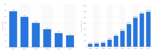
One such product that has been plagued by threat of obsolescence is the digital camera. Ever-since the invention of smartphones there has been a huge dip in the digital camera sales, as can be seen from Figure 1. The decreasing price, the exponential rate at which the pixels and the resolution of the smart-phones improved can be termed as few of the factors that cannibalized the digital camera market.

Figure 1 Worldwide Sales of Digital Cameras (2011-2016) [2] and Worldwide sale of cellphones on the right (2007-2016) [3]

1. CLUSTERING

Humans naturally use clustering to understand the world around them. The ability to group sets of objects based on similarities are fundamental to learning. Researchers have sought to capture these natural learning methods mathematically and this has birthed the clustering research. To help us solve problems at-least approximately as our brain, mathematically precise notation of clustering is important [4]. Clustering is a useful technique to explore natural groupings within multivariate data for a structure of natural groupings, also for feature extraction and summarizing. Clustering is also useful in identifying outliers, forming hypotheses concerning relationships. Clustering can be thought of as partitioning a given space into K groups i.e., 𝑓: 𝑋 → {1, …, K}. One method of carrying out this partitioning is to optimize some internal clustering criteria such as the distance between each observation within a cluster etc. While clustering plays an important role in data analysis and serves as a preprocessing step for a multitude of learning task, our primary interest lies in the ability of clusters to gain more information from the data to improve prediction accuracy. As clustering, can be thought of separating classes, it should help in classification task.

The aim of clustering is to find useful groups of objects, usefulness being defined by the goals of the data analysis. Most clustering algorithms require us to know the number of clusters beforehand. However, there is no intuitive way of identifying the optimal number of clusters. Identifying optimal clustering is dependent on the methods used for measuring similarities, and the parameters used for partitioning, in general identifying the optimal number of clusters. Determining number of clusters is often an ad hoc decision based on prior knowledge, assumptions, and practical experience is very subjective.

Get Help With Your Essay

If you need assistance with writing your essay, our professional essay writing service is here to help!
Find out more about our Essay Writing Service

This paper performs k-means and k-medoids clustering to gain information from the data structure that could play an important role in predicting obsolescence. It also tries to address the issue of assessing cluster tendency, which is a first and foremost step while carrying out unsupervised machine learning process. Optimization of internal and external clustering criteria will be carried out to identify the optimal number of cluster. Cluster Validation will be carried out to identify the most suitable clustering algorithm.

2. DATA CLEANING

Missing value in a dataset is a common occurrence in real world problems. It is important to know how to handle missing data to reduce bias and to produce powerful models. Sometimes ignoring the missing data, biases the answers and potentially leads to incorrect conclusion. Rubin in [7] differentiated between three types of missing values in the dataset:

1. Missing completely at random (MCAR): when cases with missing values can be thought of as a random sample of all the cases; MCAR occurs rarely in practice.
2. Missing at random (MAR): when conditioned on all the data we have, any remaining missing value is completely random; that is, it does not depend on some missing variables. So, missing values can be modelled using the observed data. Then, we can use specialized missing data analysis methods on the available data to correct for the effects of missing values.
3. Missing not at random (MNAR): when data is neither MCAR nor MAR. This is difficult to handle because it will require strong assumptions about the patterns of missing data.

While in practice the use of complete case methods which drops the observations containing missing values is quite common, this method has the disadvantage that it is inefficient and potentially leads to bias. Initial approach was to visually explore each individual variable with the help of “VIM”. However, upon learning the limitations of filling in missing values through exploratory data analysis, this approach was abandoned in favor of multiple imputations.

Joint Modelling (JM) and Fully Conditional Specification (FCS) are the two emerging general methods in imputing multivariate data. If multivariate distribution of the missing data is a reasonable assumption, then Joint Modelling which imputes data based on Markov Chain Monte Carlo techniques would be the best method. FCS specifies the multivariate imputation model on a variable-by-variable basis by a set of conditional densities, one for each incomplete variable. Starting from an initial imputation, FCS draws imputations by iterating over the conditional densities. A low number of iterations is often sufficient. FCS is attractive as an alternative to JM in cases where no suitable multivariate distribution can be found [8].

The Multiple imputations approach involves filling in missing values multiple times, creating multiple “complete” datasets. Because multiple imputations involve creating multiple predictions for each missing value, the analysis of data imputed multiple times take into account the uncertainty in the imputations and yield accurate standard errors. Multiple imputation techniques have been utilized to impute missing values in the dataset, primarily because it preserves the relation in the data and it also preserves uncertainty about these relations. This method is by no means perfect, it has its own complexities. The only complexity was having variables of different types (binary, unordered and continuous), thereby making the application of models, which assumed multivariate normal distribution- theoretically inappropriate. There are several complexities that surface listed in [8]. In order to address this issue – It is convenient to specify imputation model separately for each column in the data. This is called as chained equations wherein the specification occurs at a variable level, which is well understood by the user.

The first task is to identify the variables to be included in the imputation process. This generally includes all the variables that will be used in the subsequent analysis irrespective of the presence of missing data, as well as variables that may be predictive of the missing data. There are three specific issues that often come up when selecting variables:

(1) creating an imputation model that is more general than the analysis model,

(2) imputing variables at the item level vs. the summary level, and

(3) imputing variables that reflect raw scores vs. standardized scores.

To help make a decision on these aspects, the distribution of the variables may help guide the decision. For example, if the raw scores of a continuous measure are more normally distributed than the corresponding standardized scores then using the raw scores in the imputation model, will likely better meet the assumptions of the linear regressions being used in the imputation process.

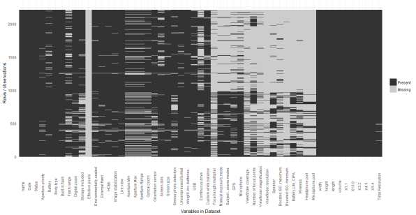
The following image shows the missing values in the data-frame containing the information regarding digital camera.

Figure 2 Missing Variables

We can see that “Effective Pixels” has missing values for all its observations. After cross verifying it with the source website, the web scrapper was rewriting to correctly capture this variable from the website. The date variable was converted from a numeric to a date and this enabled the identification of errors in the observation for “USB” in the dataset. Two cameras that were released in 1994 & 1995 were shown to have USB 2.0, after searching online, it was found out that USB 2.0 was released in the year 2005 and USB 1.0 was released in the year 1996. As, most of the cameras before 1997 used PC-serial port a new level was introduced to the USB variable to indicate this.

3. DATA DESCRIPTION

The dataset containing the specification of the digital cameras was acquired using “rvest -package [5]” in R from the “url” provided in [6]. The structure of the data set is as shown in Appendix A. The data-frame contains 2199 observation and 55 variables. Appendix B contains the descriptive statistics of the quantitative variables in the data-frame.

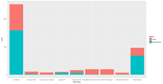
Figure 4 The Distribution of Body-Type in the dataset

Observation: Most of the compact, Large SLR and ultracompact cameras are discontinued.

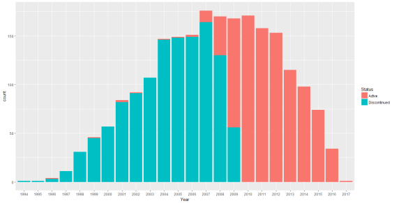
Figure 5 Plot showing the status of Digital Cameras from 1994-2017

Observation: Most of the cameras released before 2007 have been discontinued however, we can see that few cameras announced between the period of 1996-2006 are still in production. Fewer new cameras have been announced after the year 2012, this can be evidenced due to the decreasing number of camera sales presented in Figure 5.

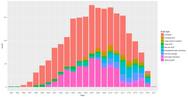
Figure 6 Distribution of different Cameras (1994-2017)

Observation: Between the period of 1996 – 2012 the digital camera market was dominated by the compact cameras. After 2012, fewer new compact cameras have been announced or are still in production. Same can be said about the fate of ultracompact cameras. In the year 2017, only SLR – style mirrorless cameras have been announced, signaling the death of point and shoot cameras.

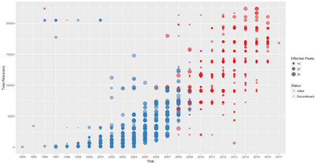
Figure 7 Plot showing the Change in the Total Resolution and Effective Pixels of Digital Camera over the Years

Observation: Total resolution has seen an improvement over the years. The presence of outliers can be seen in the top-left corner of the plot. Although the effective pixel is around 10, the total resolution is far higher than any of the cameras announced between the period 1996-2001. These could be the cameras that are still in production as evidenced from Figure 7.

4. ASSESSING CLUSTER TENDENCY

A primary issue with unsupervised machine learning is the fact if carried out blindly, clustering methods will divide the data into clusters, because that is what they are supposed to do. Therefore, before choosing a clustering approach, it is important to decide whether the dataset contains meaningful clusters. If the data does contain meaningful clusters, then the number of clusters is also an issue that needs to be looked at. This process is called assessing clustering tendency (feasibility of cluster analysis).

To carry out a feasibility study of cluster analysis Hopkins statistic will be used to assess the clustering tendency of the dataset. Hopkins statistic assess the clustering tendency based on the probability that a given data follows a uniform distribution (tests for spatial randomness). If the value of the statistic is close to zero this implies that the data does not follow uniform distribution and thus we can reject the null hypothesis. Hopkin’s statistic is calculated using the following formula:

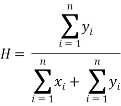
Where x_i is the distance between two neighboring points in a given, dataset and y_i represents the distance between two neighboring points of a simulated dataset following uniform distribution. If the value of H is 0.5, this implies that and are close to one another and thus the given data follows a uniform distribution. The next step in the unsupervised learning method is to identify the optimal number of clusters.

The Hopkins statistic for the digital camera dataset was found to be “0.00715041”. Since Hopkins statistic was quite low, we can conclude that the dataset is highly clusterable. A visual assessment of the clustering tendency was also carried out and the result can be seen in Figure 8.

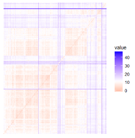
Figure 8 Dissimilarity Matrix of the dataset

5. DETERMINING OPTIMAL NUMBER OF CLUSTERS

One simple solution to identify the optimal number of cluster is to perform hierarchical clustering and determine the number of clusters based on the dendogram generated. However, we will utilize the following methods to identify the optimal number of clusters:

1. An optimization criterion such as within sum of squares or Average Silhouette width
2. Comparing evidence against null hypothesis. (Gap Statistic)

1. SUM OF SQUARES

The basic idea behind partitioning methods like k-means clustering algorithms, is to define clusters such that the total within cluster sum of squares is minimized.

Where C_k is the k^th cluster and W(C_k) is the variation within the cluster. Our aim is to minimize the total within cluster sum of squares as it measures the compactness of the clusters.

In this approach, we generally perform clustering method, by varying the number of clusters (k). For each “k” we compute the total within sum of squares. We then plot the total within sum of squares against the k-value, the location of bend or knee in the plot is considered as an appropriate value of the cluster.

2. AVERAGE SILHOUETTE WIDTH

Average silhouette is a measure of the quality of clustering, in that it determines the how well an object lies within its cluster. The metric can range from -1 to 1, where higher values are better.

Average silhouette method computes the average silhouette of observations for different number of clusters. The optimal number of clusters is the one that maximizes the average silhouette over a range of possible values for different number of clusters [9].

Average silhouette functions similar to within sum of squares method. We carry out the clustering algorithm by varying the number of clusters, then we calculate average silhouette of observation for each cluster. We then plot the average silhouette against different number of clusters. The location with the highest value of average silhouette width is considered as the optimum number of cluster.

3. GAP STATISTIC

This method compares the total within sum of squares for different number of cluster with their expected values while assuming that the data follows a distribution with no obvious clustering.

The reference dataset is generated using Monte Carlo simulations of the sampling process. For each variable (x_i) in the dataset we compute its range [min(x_i), max(x_j)] and generate n values uniformly from the range min to max.

The total within cluster variation for both the observed data and the reference data is computed for different number of clusters. The gap statistic for a given number of cluster is defined as follows:

denotes the expectation under a sample of size n from the reference distribution. is defined via bootstrapping and computing the average . The gap statistic measures the deviation of the observed W_k value from its expected value under the null hypothesis.

The estimate of the optimal number of clusters will be a value that maximizes Gapn(k). This implies that the clustering structure is far away from the uniform distribution of points.

The standard deviation (sdk) of is also computed in order to define the standard error s_k as follows:

Finally, we choose the smallest value of the number of cluster such that the gap statistic is within one standard deviation of the gap at k+1

Gap(k)≥Gap(k+1) – s_k+1

The above method and its explanation are borrowed from [10].

6. DATA PRE-PROCESSING

The issue with K-means clustering is that it cannot handle categorical variables. As the K-means algorithm defines a cost function that computes Euclidean distance between two numeric values. However, it is not possible to define such distance between categorical values. Hence, the need to treat categorical data as numeric. While it is not improper to deal with variables in this manner, however categorical variables lose their meaning once they are treated as numeric.

To be able to perform clustering efficiently, Gower distance will be used for clustering. The concept of Gower distance is that for each variable a distance metric that works well for that particular type of variable is used. It is scaled between 0 and 1 and then a linear combination of weights is calculated to create the final distance matrix.

7. PARTITIONING METHODS

1. K-MEANS

K-means clustering is the simplest and the most commonly used partitioning method for splitting a dataset into a set of k clusters. In this method, we first choose K initial centroids. Each point is then assigned to the closest centroid, and each collection of points is assigned to a centroid in the cluster. The centroid of each cluster is updated based on the additional points assigned to the cluster. We repeat his until the centroids find a steady state.

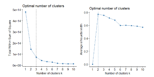
Figure 9 Plot Showing total sum of square and Average Silhouette width for different number of clusters

We can see from Figure 9, that the optimal number of clusters suggested by the optimization criteria is 3 clusters using WSS method and 2 clusters using Average Silhouette width method.

Considering the dependent variable is factor with two levels, having two clusters does make sense. The disadvantage of optimization criterion to identify the optimal clusters is that, it is sometimes ambiguous. A more sophisticated method is the gap statistic method.

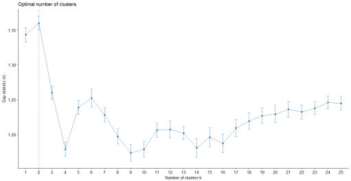
Figure 10 Gap Statistic for different number of clusters

From Figure 10, we can see that the Gap statistic is high for 2 clusters. Hence, we carry out k-means clustering with 2 clusters on a majority basis.

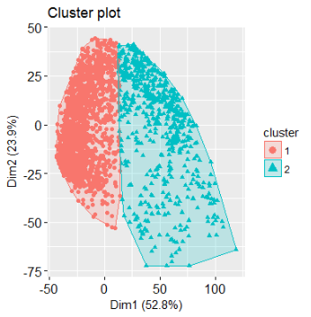
Figure 11 Visualizing K-means Clustering Method

The data separates into two relatively distinct clusters, with the red category in the left region, while the region on the right contains the blue category. There is a limited overlap at the interface between the classes. To visualize K-means it is necessary to bring the number of dimensions down to two. The graph produced by “fviz_cluster: Factoextra Ver: 1.0” [11] is not a selection of any two dimensions. The plot shows the projection of the entire data onto the first two principle components. These are the dimensions which show the most variation in the data. The 52.8% indicates that the first principle component accounts for 52.8% variation in the data, whereas the second principle component accounts for 23.9% variation in the data. Together both the dimensions’ account for 76.7% of the variation. The polygon in red and blue represent the cluster means.

2. PARTITIONING AROUND MEDOIDS

K – means clustering is highly sensitive to outliers, this would affect the assignment of observations to their respective clusters. Partitioning around medoids also known as K-medoids clustering are much more robust compared to k-means.

K-medoids is based on the search of medoids among the observation of the dataset. These medoids represent the structure of the data. Much like K-means, after finding the medoids for each of the K- clusters, each observation is assigned to the nearest medoid. The aim is to find K-medoids such that it minimizes the sum of dissimilarities of the observations within the cluster.

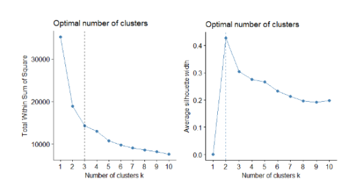
Figure 12 Plot Showing total sum of square and Average Silhouette width for different number of clusters

We can see from Figure 12, that the optimal number of clusters suggested by the optimization criteria is 3 clusters using WSS method and 2 clusters using Average Silhouette width method. Considering the dependent variable is factor with two levels, having two clusters does make sense. The disadvantage of optimization criterion to identify the optimal clusters is that, it is sometimes ambiguous. A more sophisticated method is the gap statistic method.

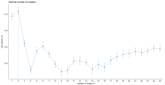
Figure 13 Gap Statistic for different number of clusters

From Figure 13, we can see that the Gap statistic is high for 2 clusters. Hence, we carry out partitioning around medoids clustering with 2 clusters on a majority basis.

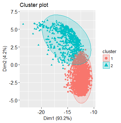
Figure 14 Plot visualizing PAM clustering method

The data separates into two relatively distinct clusters, with the red category in the lower region, while the upper region contains the blue category. There is a limited overlap at the interface between the classes. “fviz_cluster: Factoextra Ver: 1.0” [11] transforms the initial set of variables into a new set of variables through principal component analysis. This dimensionality reduction algorithm operates on the 72 variables and outputs the two new variables that represent the projection of the original dataset.

8. CLUSTER VALIDATION

The next step in cluster analysis is to find the goodness of fit and to avoid finding patterns in noise and to compare clustering algorithms, cluster validation is carried out. The following cluster validation measures to compare K-means and PAM clustering will be used:

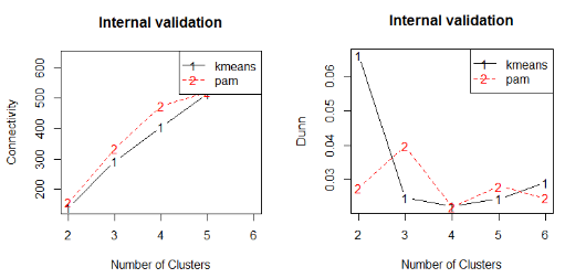
• Connectivity: Indicates the extent to which the observations are placed in the same cluster as their nearest neighbors in the data space. It has a value ranging from 0 to ∞ and should be minimized
• Dunn: It is the ratio of shortest distance between two clusters to the largest intra-cluster distance. It has a value ranging from 0 to ∞ and should be maximized.
• Average Silhouette width

The results of internal validation measures are presented in the table below. K-means for two cluster has performed better for each statistic.

Figure 15 Plot Comparing Connectivity and Dunn Index for K-means and PAM for different number of clusters     

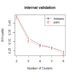
Figure 16 Plot Comparing Average Silhouette width of K-means and PAM

Table 1 Presenting the values of different validation measures for K-means and PAM

Table 2 Optimal Scores for the Validation Measures

9. CONCLUSION

In this research work, partitioning methods like K-means and Partitioning around medoids were developed. The performances of these two approaches have been observed on the basis of their Connectivity, Dunn index and Average Silhouette width. The results indicate that K-means clustering algorithm with K = 2 performs better than partitioning around medoids with two clusters. The findings of this paper will be very useful to predict obsolescence with higher accuracy.

10. FUTURE WORK

Advanced clustering algorithms such as Model based clustering and Density based clustering can be carried out to find the multivariate data structure as most of the variables are categorical.

[1] Bjoern Bartels, Ulrich Ermel, Peter Sandborn and Michael G. Pecht (2012). Strategies to the Prediction, Mitigation and Management of Product Obsolescence.

[2] Source Figure 1: https://www.statista.com/statistics/269927/sales-of-analog-and-digital-cameras-worldwide-since-2002/

[3] Source, Figure 1: https://www.statista.com/statistics/263437/global-smartphone-sales-to-end-users-since-2007/

[4] S. Still, and W. Bialek, “How many Clusters? An Information Theoretic Perspective”, Neural Computation, 2004.

[5] Wickham, Hadley, “rvest: Easily Harvest (Scrape) Web Pages”. https://cran.r-project.org/web/packages/rvest/rvest.pdf, Ver. 0.3.2

[6] https://www.dpreview.com

[7] Rubin, D.B., Inference and missing data. Biometrika, 1976.

[8] “Multivariate Imputation by Chained Equations” – Stef van Buuren, Karin Groothuis .

[9] “Learning the k in k-means” Greg Hamerly, Charles Elkan

[10] Robert Tibshirani, Guenther Walther and Trevor Hast