Equation to Model a Cooling Cup of Coffee

MATHEMATICS SL Internal Assessment

Mathematically Determining an Equation to Model a Cooling Cup of Coffee

I. Introduction

After having spent countless hours completing assignments and projects, I have too often found my coffee to be cold by the time I get around to drinking it. As a result, I began to question the reasoning behind such. Thus I drew inspiration to tackling this particular task, as my confusion greatly intrigued me to explore such a question. After learning about the depths of calculus and the various applications of the math, I wanted to apply what I had explored in class to something that was physical and relevant in order to justify that what I was learning was applicable towards the everyday life. After some considerations, I decided on the topic of coffee.

From taking my higher level chemistry course in school, I knew that the difference between the cooling body and the ambient temperature – specifically the temperature of the room – changed at the rate at which the body cooled. Consequently, I realized that large differences between temperatures of the cooling body and ambient temperature caused a large rate of change, with smaller differences caused a smaller rate of change (Feldman, 2011). From common knowledge I figured that the equation being modelled would be seen as an exponential curve, as I knew the coffee would not be able to reach points below room temperature, which ultimately meant that the coffee would instead approach room temperature with the rate of change simultaneously becoming smaller and smaller. In this situation, the difference between the ambient and body temperature would change accordingly (Feldman, 2011). After taking such pre-calculations into consideration, I set the objective to create a model of the rate of cooling and then produce an equation from such in order to calculate how long I would be able to revisit my coffee until the point at which it became undrinkable. My biggest goal for this investigation was to be able to solve an equation that would allow me to produce a value that bore significance in the real world, specifically to others facing the same issue.

II. Data Collection

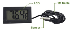
Prior to producing a graph, I needed to first collect the data regarding the cooling of a cup of coffee over a series of minutes. The data shown below was achieved using a temperature sensor and mobile stopwatch that produced a set of readings measuring the temperature of the coffee to 1.d.p per 5 seconds for 2 hours. I repeated this three times in three distinct trials in order to obtain a sufficient set of data readings. The recordings are listed below.

Experimentally Determined Values of the Temperature of the Coffee (℃) Over a Fixed Period of Time (Two Hours) Through a Series of Five Minutes Intervals

Figure 1.0: Table of Values Indicating the First Trial of Results

Figure 1.1: Table of Values Indicating the Second Trial of Results

Figure 1.2: Table of Values Indicating the Third Trial of Results

As can be depicted through the above tables, the results as collected did not vary so much; and the overall data set remained fairly the same. Nevertheless, I averaged out each data set for each specific time slot between the three trials using the formula:

$\underline{x}=\frac{\sum _{}^{}\left(x\right)}{n}$

,

where $\underline{x}$

indicates the mean;

$\sum _{}^{}\left(x\right)$

indicates the sum of data values,

and $n$

indicates the number of data values

II. Data Processing

 After the data was collected in the tables and averaged out between each trial, as shown above, the next stage logically was to graph the results and produce a graph of my own. The scatter plot below was produced using Microsoft Excel, with the time in minutes (over 5 minute intervals) – in the graph the scale was deduced to 20 minute intervals -  plotted on the X axis and the temperature (℃) plotted on the Y axis. The graph below thus indicates the experimentally determined values of the temperature of the coffee over a series of two hours (with the result

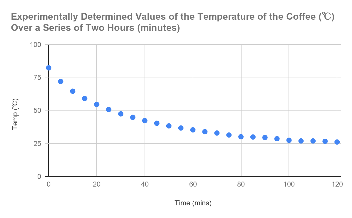
Figure 1.3: Graph displaying the change in temperature of the coffee in relation to time.

As can be seen in the above figure, the graph shows an exponential curve, between the values of temperature of the coffee and the time in minutes.

From this it could be assumed:

The power of the exponential is negative:

The graph thus holds a negative correlation, so logically it would mean that the power of the function must be negative.

When time (t) = 0, Temperature (T) = 83.2:

The y-intercept, which correlates to the initial temperature of the tea, is 83.2℃.

The room temperature is 24.0℃:

The tea can never go below this temperature.

From these observations, I built a formula of the curve displayed above. I chose the power $e$

to solve the equation later after having determined the constants.

The graph displayed an exponential decay relation:

$T =e{–t}^{}$

Due to the temperature of the room being 24℃, the entire graph was translated up the y axis by a degree of 24, and thus there was a translation constant:

$T=\mathit{Tc} + e{–t}^{}$

(where $\mathit{Tc}$

= 24, representing the ambient temperature)

To translate this equation to represent the original, it requires a translation on the x axis (k) and a gradient much smaller 1(a), so it can be assumed that:

There is a stretch constant on the x-axis (a), where 1 > a > 0

$T=T{c + e{–t}^{}}_{}$

There is a translation constant on the y-axis (k)

$T=\mathit{Tc} +\mathit{ke}{–\mathit{at}}^{}$

This section of the investigation caused some mayhem, as I had a lot of issues within this particular area of the report. I had produced an equation and had found it difficult to solve it.

As a first step, I rearranged the formula using natural logs:

*Note: $\mathit{ln} \left(e\right) =1$

*

$T=\mathit{Tc} +\mathit{ke}{–\mathit{at}}^{}$

$T–\mathit{Tc}=\mathit{ke}{–\mathit{at}}^{}$

$\mathit{ln} (T–\mathit{Tc}) =\mathit{ln} \left(\mathit{ke}{–\mathit{at}}^{}\right)$

$\mathit{ln} (T–\mathit{Tc}) =\mathit{ln} \left(k\right) + \mathit{ln} (–\mathit{at}) \times \mathit{ln} \left(e\right)$

Following this step, I let $t=0$

and 83.2 degrees and $t=60$

and 35.4 degrees. I then used two results from the data to create a pair of two variable equations where $\mathit{Tc} =24.$

$\mathit{ln} (83.2 – 24) = \mathit{lnk} – 0a$

(Equation A)

$\mathit{ln} (35.4– 24) = \mathit{lnk} – 60a$

(Equation B)

*Subtract Equation A from Equation B*

$\mathit{ln} (11.4) – \mathit{ln} (59.2) = (\mathit{lnk} – \mathit{lnk}) –60a$

$\mathit{ln} (11.4) – \mathit{ln} (59.2)= –60a$

$\mathit{ln} (\frac{11.4}{59.2}$

) = -60a

$\frac{1.6}{–60}$

= a

$a=–0.0274$

Solving for variable k:

$\mathit{ln} (83.2– 24) =\mathit{lnk} – (0\times –0.0274)$

$\mathit{ln} (59.2) =\mathit{lnk}$

$59.2 =k$

Final Equation:

$T=24 + 59.2e{–0.0274t}^{}$

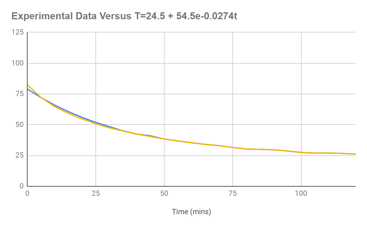
The final equation produced seems to produce a graph that matches the original data, but it can be seen with the results that the rate of cooling in the first 50 seconds of cooling is underpredicted. $T=24 + 59.2e{–0.0274t}^{}$

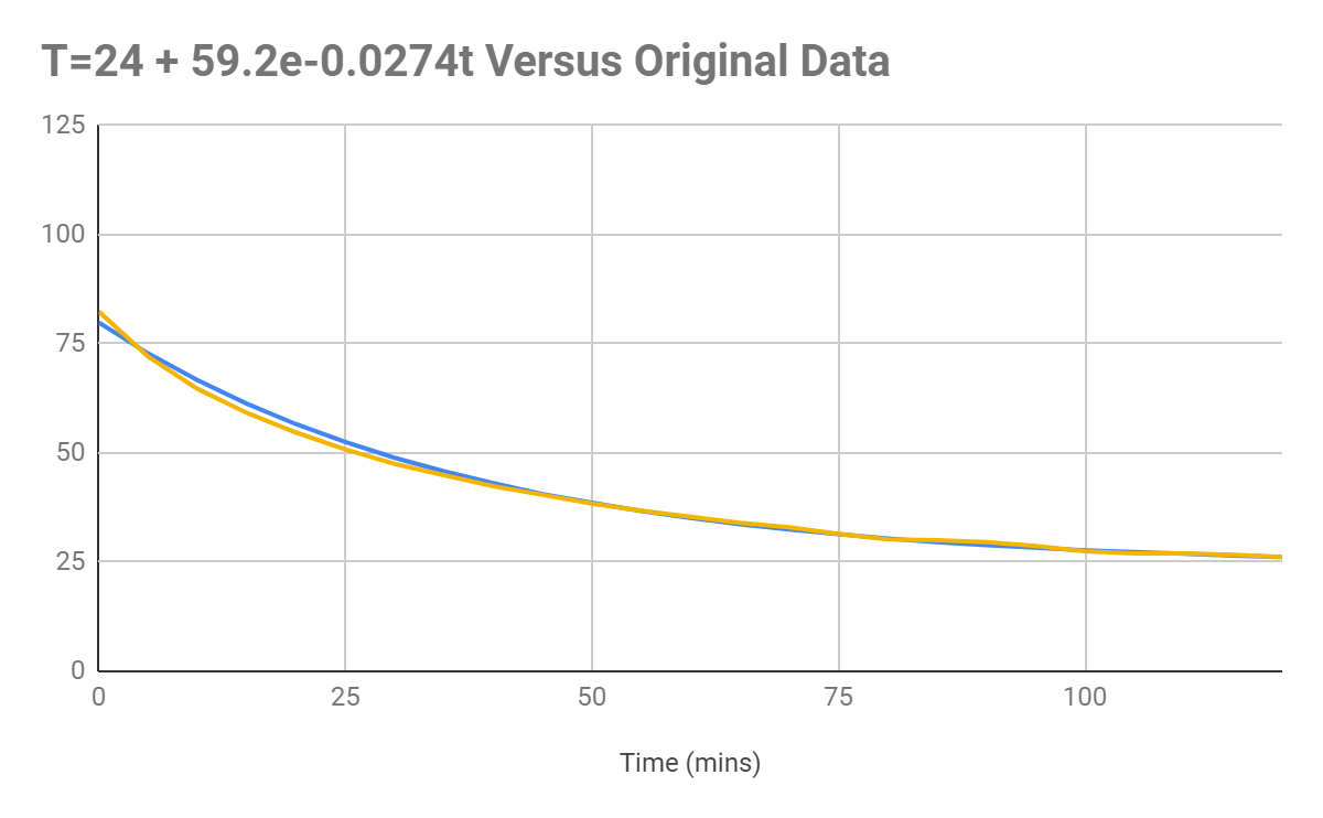
It can be seen from the graph that the actual data (orange) tends to be slightly lower than the temperature projected by the original data. I believe that this could

have been caused by the method used not accounting for the

Figure 1.4: Graph displaying the data as graphed according to $T=24 + 59.2e{–0.0274t}^{}$

(orange) versus the original data (blue).

anomalies in the data. To try and produce a more accurate series; however, and one that accounts for the natural errors in the data lines of best fit could be used to produce a model of the curve. In order to create a formula that accounted for the uncertainties, I started to look at the equation in a more representative fashion, the exponential is very difficult  to solve in its original form, but linear graphs are a lot easier to solve. With some guidance I simplified the equation again using logs until it represented something similar to $y=\mathit{mx} + b.$

Initial Equation:

$T\left(t\right) = \mathit{Tc} +\mathit{ke}{–\mathit{at}}^{}$

$T\left(t\right) – \mathit{Tc} =\mathit{ke}{–\mathit{at}}^{}$

$\mathit{Ln} (T – \mathit{Tc}) =\mathit{Ln} \left(\mathit{ke}{–\mathit{at}}^{}\right)$

$\mathit{Ln} (T – \mathit{Tc}) =\mathit{Ln} \left(k\right) – \mathit{atLn}\left(e\right)$

$\frac{\left|\mathit{Ln} \right(T – \mathit{Tc}\left)\right|}{y} =\frac{ |–\mathit{at}|}{\mathit{mx}} – \frac{\left|\mathit{atLn}\right(e\left)\right|}{b}$

$y=\mathit{mx} +b$

From this I used the experiment data to plot the graph of $\mathit{Ln} (T–\mathit{Tb})$

on excel, producing the following straight line from the graph.

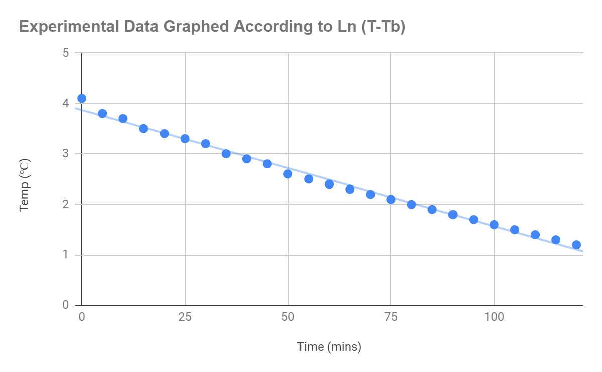
Figure 1.5: Graph displaying a linear correlation according to the equation $\mathit{Ln} (T–\mathit{Tb})$

, when applied to the original experimental data                                                                                                                                                   

The line, as depicted through the graph, can be seen to be accounted for small uncertainties in the line created by real world factors. The equation for the line of best fit was generated:

$y= –0.0298x + 3.9872$

Through applying the $y=\mathit{mx} +b$

formula, it can be denoted that:

$y= –0.0298x + 3.9872$

If you work backwards, they will correspond to:

$\frac{\left|\mathit{Ln} \right(T – \mathit{Tc}\left)\right|}{y} =\frac{ |–\mathit{at}|}{\mathit{mx}} – \frac{\left|\mathit{atLn}\right(e\left)\right|}{b}$

So that $\mathit{Ln} \left(k\right) =3.9872$

$–a =–0.0298$

$x=t$

From here k can be solved:

$e{3.9872}^{} =k$

$53.9 =k$

Thus the equation $T=24 + 54.5e{–0.0298t}^{}$

is produced.

As can be seen below, the data are basically identical, with the only difference being that the equation generated values intersect the y-axis at a lower value. The asymptote is the same, with the mean error of the differences in values being 0.11℃.

Figure 1.6: Graph displaying the original data versus the original data graphed according to the equation $T=24.5 + 54.5e{–0.0274t}^{}$

Although seemingly accurate, I wanted to further explore and delve into the actual math of Newton’s law of cooling, as stated in the introduction, which states that:

The rate of change of the temperature $\frac{\mathit{dT}}{\mathit{dt}}$

, is directly proportional to the difference between the temperature of the soup T(t) and the ambient temperature $\mathit{Tc}.$

( $\frac{\mathit{dT}}{\mathit{dt}}$

,= (T-Tc).

According to online publications, integration was used through Newton’s law of cooling, and the fact that $\mathit{Tc}$

(original temperature) is a constant can be used to convert the above integral into a $y=\mathit{mx}+b$

equation, with the resulting equation being (Murray, 2012):

$T\left(t\right) =\mathit{Tb} +(\mathit{Td}–\mathit{Td})e{\mathit{kt}}^{}$

$T=\mathit{temperature}$

$\mathit{Td}=\mathit{ambient} \mathit{temperature}$

$t=\mathit{time}$

$k=\mathit{constant}$

Factoring into such conditions and using $\frac{\left|\mathit{Ln} \right(T – \mathit{Tc}\left)\right|}{y} =\frac{ |–\mathit{at}|}{\mathit{mx}} – \frac{\left|\mathit{atLn}\right(e\left)\right|}{b}$

, I generated such an equation:

$T\left(t\right) =24 +(54.5)e{–0.0274t}^{}$

Graphing $T\left(t\right) =24 +(54.5)e{–0.0274t}^{}$

this is produced:

As indicated through the graph, the two lines are basically identical, and the equation produced greatly resembles the first equation produced.                                      Figure 1.7: Original data compared to $T\left(t\right) =24 +(55.9)e{–0.0279t}^{}$

.

Comparison of Results

III. Conclusion and Evaluation

*This is compared to the original recorded data from the experiment conducted.*

The average error, here given as the absolute error, shows that 2nd equation is more consistently similar to the original value produced by the graph.The least accurate would be 1st equation, despite it having been produced through a virtually identical method to 3rd equation. This is thought to be due to the values that were selected to be used in the equation, as the real data produced some discrepancies to Newton’s law of cooling, as a result of changes in real world factors (ambient temperature for example) (Murray, 2012).

It can be seen that the second equation, which was produced using lines of best fit, produced the most accurate model of the coffee cooling down.This is most likely due to the fact that the lines of best fit take into account the slight discrepancies  in the real results that were caused by the environment. Since the third and first equation rely on the fact that $\mathit{Ta}$

is always equal to 24.5, there could have been major inaccuracies as as the coffee cooled down, the air surrounding it would have immediately warmed up as the heat diffused away from the cup (Murray, 2012). This then explains why the differences of the first and third equation were so great, as between the two, a lower ambient temperature was always predicted, thus inaccurately assuming that the rate of change was faster.

To answer my original research question, “How long can I revisit my coffee before it becomes undrinkable?”, I can achieve this by using the second equation:

$T=24 + 54.5e{–0.0298t}^{}$

Assuming that 30℃ is an undrinkable temperature,

$30=24 + 54.5e{–0.0298t}^{}$

$30 –v=24 + 54.5e{–0.0298t}^{}$

$t=84.6 \mathit{minutes}$

I can safely revise that 1.41 hours will be the proper time before my coffee is undrinkable. As precise as this value is however, it only represents how long I can leave my coffee out in a room with 24℃ temperature. A second investigation would be interesting to see if an equation could be produced that takes into account the surface area of the cooling body and the changing ambient temperature.

However, with the equation produced above, despite the discrepancies, it represents an extremely accurate model of the cooling coffee. Thus I have fulfilled my objective of determining an equation to model the cup of cooling coffee through implementing the laws of logarithms and simultaneous equations. Through this investigation, I was able to apply math to a real life situation outside of the classroom environment.

IV. Works Cited

• Feldman, Joel, et al. “CLP-1 Differential Calculus.” Plimpton 322, www.math.ubc.ca/~CLP/CLP1/clp_1_dc/sec_newtonCooling.html.
• “Newton’s Law of Cooling.” Math24, www.math24.net/newtons-law-cooling/.
• Bourne, Murray. “3. The Logarithm Laws.” Intmathcom RSS, www.intmath.com/exponential-logarithmic-functions/3-logarithm-laws.php.
• “Exponential Decay.” From Wolfram MathWorld, mathworld.wolfram.com/ExponentialDecay.html.