Geostatistics and Advance Reservoir Modelling Essay

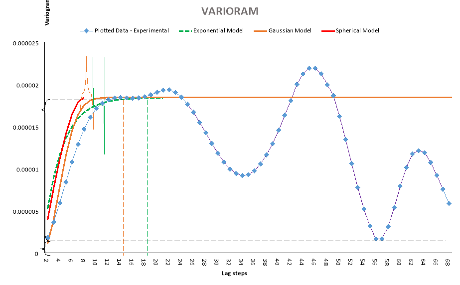
Figure 1. All models are based on equations (next page) and plotted manually in excel to show their respective behavior. Spherical model fails to proceeds as lag exceed the practical range.

Modelling and Interpreting Variogram

Jahanzeb Ahsan (8529193) B.Eng Petroleum Engineering

Introduction

There are a dozen different variogram models. Four most frequent used are:

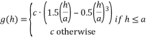
1. Spherical: Smooth behavior at origin and more linear.

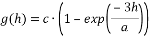
2. Exponential: Greater slope than spherical i.e. relates to more random variables than spherical model.

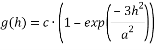
3. Gaussian: Using only Gaussian in absence of nugget can lead to problems in Kriging.

4. Power: Also associated with fractal models.

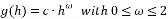
For above equations ‘h’ shows lag distance, ‘a’ is the practical range and ‘c’ is sill.

There are three basic terms in all variograms; sill, nugget and range, as shown in figure 1. Sill is the value obtained after stabilizing the experimental curve by fitting a variogram model. It signifies ‘zero’ or no correlation of our spatial data, since variogram can be imagined as an inverse of variance graph, the sill shows the maximum variance i.e. there is no distance (zero lag) between the data, hence maximum correlation (for variance). Range is said to be the maximum distance for which correlation between 2 points can exist – beyond this autocorrelation cease to working – In terms of geology vertical range is greater than horizontal range due to difference in scale, ‘geometric anisotropy’. When comparing a horizontal variogram with vertical having different sills but same range one may conclude it as a ‘zonal anisotropy’, often due to stratification and layering. Range can also varies with type of model used. Based on the model equation figure 1 shows a manual attempt to demonstrate Gaussian model reaches sill (range is at lag 14) before exponential model having greater range (at lag 18). Range is said to be directionally dependent if anisotropy exist – geology is more anisotropic vertically than laterally. Nugget is an unavoidable error at origin in data. No correlation in data can lead to ‘Pure Nugget’, an ideal model have zero-nugget. For ease of understanding one can term it as an inherited error e.g. from measuring instruments. Figure 1 shows a nugget of 1.7732E-06.

Noise can appear due to lack of data pairs and is more prominent in directional variogram, hence they do not show overwhelming evidence of anisotropy. Pure nugget models are also known as ‘white noise’ i.e. the data shows no spatial correlation.

Interpreting Experimental Variogram (figure 1)

For variogram or any other geostatistical method precision and optimality increases when the data is stationary and normally distributed i.e. mean and variance does not vary considerably. High deviation from data normality and stationary can result in complications.

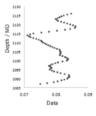
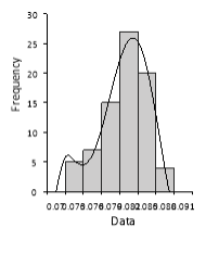
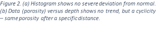
A skewed histogram influence the durability in estimation of variogram. Similarly if theoretical sill (see figure 1) is below experimental variogram a trend in data exist, which should be removed before interpreting the experimental variogram, however this does not mean it will solve the problem – no trend in dataset, see figure 2 (b). In other words geological data like porosity, grain size and permeability often shows trend which result in negative correlation as distance increases resulting in variogram to exceed sill (not in this case).

Cyclicity (geological cyclicity) also known as hole-effect is another important phenomenon variograms exhibit (purple line, see figure 1). Periodic repeated variations like facies and other physical properties yield a cyclic behavior on variogram and like in figure 1 cause the variogram to deviate (below sill in this case). Cyclicity often diminishes over increasing distance as these periodic repeated geological variations are not consistent. This hole-effect phenomenon maybe insignificant in terms of overall variance but nonetheless should be included in a variogram’s interpretation.

Table 1 shows the skewness as negative, however not perfectly skewed, however one can assume it due to lack of data since our range of measurement is only 39 f.t. Table 1 concludes our data is not perfectly normally distributed, hence our variogram model and Kriging will be affected significantly.

Table 1. Basic statistical analysis of data

Conclusion

• A real variogram consist of all or combination of features such as hole-effect, sill, range, an experimental data set fitted with appropriate model.
• Variograms such as rodograms or modograms or relative pairwise variograms are used when simple variograms fail to detect anisotropy and range.
• Amount if data is a big constraint in variogram modeling such that bigger the data, more accurate model.
• Spherical model fail to fit when lag distance exceed the practical range (like in our case).
• Lack of appropriate software and manual input of model equation in excel shows an approximate guide to how spherical, exponential and Gaussian model will behave. Gaussian model gives the best fit model and least nugget effect.
• A trend and sparseness in data greatly degrades the authenticity of variogram.
• Often biased especially when modelled inaccurately.

Despite having its disadvantages a variogram can be a useful tool in heterogeneity analysis; an indicator variogram which converts the values into 1s and 0s is notably useful in quantification of lithological and geological units and future predictions. Kriging interpolation technique uses variogram.

References

Bohling, G., 2007. In: INTRODUCTION TO GEOSTATISTICS. Boise: Boise State University, pp. 15-25.

Dubrule, O., 1998. Geostatistics in Petroleum Geology. Tulsa: American Association of Petroleum Geologists.

Emmanuel Gringarten, C. V. D., 2001. Teacher’s Aide Variogram Interpretation and Modeling. Mathematical Geology, 33(4), pp. 507-534.

Fanchi, J. R., 2006. Principles of Reservoir Simulation. 3rd ed. Oxford: Elsevier B.V.

Gregoire Mariethoz, J. C., 2014. Multiple-point geostatistics. 1st ed. s.l.: John Wiley & Sons, Ltd.

Hodgetts, D. D., 2014. Geostatistics and Stochastic Reservoir Modelling. Manchester: s.n.

Huihui Zhang, Y. L. R. E. L. Y. H. W. C. H. D. M. G. C., 2009. Analysis of variograms with various sample sizes from a multispectral image. Int J Agric & Biol Eng , 2(4), pp. 62-69.

M. J. Pyrcz, C. V. D., n.d. The Whole Story on the Hole Effect. [Online] Available at: http://ceadserv1.nku.edu/longa//mscc/boyce/gaa_pyrcz_deutsch.pdf [Accessed 9 November 2014].