Effects of Cargo Ship Traffic on Underwater Decibel Levels
| ✅ Paper Type: Free Essay | ✅ Subject: Geography |
| ✅ Wordcount: 2908 words | ✅ Published: 23 Sep 2019 |
IB internal assessment: Analyzing the Effects of Cargo Ship Traffic on Underwater Decibel Levels
Identifying the context
Most humans rely on the sense of sight as their primary means of measuring distance. In contrast, cetaceans use biosonar, or echolocation. Echolocation is the process by which cetaceans emit noises to create reflected sound, or echoes, off targets. Cetaceans typically exert low frequency waves (30-60 kHZ), as in optimal conditions, such waves travel great distances[1]. These echoes inform cetaceans of target locations, if they are moving, and the size of the objects[2]. It is believed primal whales evolved 50 million years ago, along with this technique[3].
Humans have been identified as the point source of the drastic reduction of distance that cetaceans can rely on, when using echolocation. Along with the industrial revolution and other momentous periods of expansion and development, the soundscape of the oceans changed for the worse. Large cargo ships can significantly reduce the maximum echolocation range due to their sizable engines and forceful propellers pushing through the water[4]. Not only do they create noise while treading through the water, but the bubbles produced by the sloshing wake pop and increase the decibel level of the soundscape. The low frequency waves originating from the ships’ engines and propellers travel incredibly well through water, that they may raise the noise levels of the ocean by a large amount[5]. Although the exact distance a whale needs to communicate is presently unknown, this increasingly noisy soundscape could affect their ability to find a mate, feed, navigate, and keep track of their young[6]. In modern times with the increased noise levels, when a whale signals they may only be witnessed from a short distance due to human interference through shipping.
The National Oceanic and Atmospheric Administration (NOAA) is working towards the goal of eliminating noise, caused by human activity, alongside independent non-profits, such as The Oceanic Preservation Society. Strict regulations have been instated, and a timeline has been laid out for the transition of the soundscape to its state prior to the industrial revolution.
Research Question
To what extent have humans impacted the noise levels (measured in decibels) of the Atlantic Ocean, Gulf of Mexico, and Gulf of California through shipping activity when comparing 2002 to 2004, as measured through the use of hydrophones?
Justification
Scientists have noticed a colossal difference in animals’ habits though the past century due to the soundscape in the oceans changing[7]. This change has been attributed, in part, to the more than 17,000 cargo ships that sail daily[8]. Low frequency waves from cetaceans that could have been heard hundreds of miles away are now being drowned out by ships, only to be heard as little as less than a mile away[9]. It is known that ships affect the marine ecosystems by polluting sound, but it is unclear to what extent.
Variables
Independent:
- Time (years)
Dependent:
- Sound measured from hydrophones (decibels)
Controlled:
- Location
- Hydrophones
Materials
- Computer (to analyze the data)
Procedure
Part 1
-
Obtain maps of decibel levels of the Atlantic Ocean, Gulf of Mexico, and Gulf of California from 2002 and 2004.
Figure 1
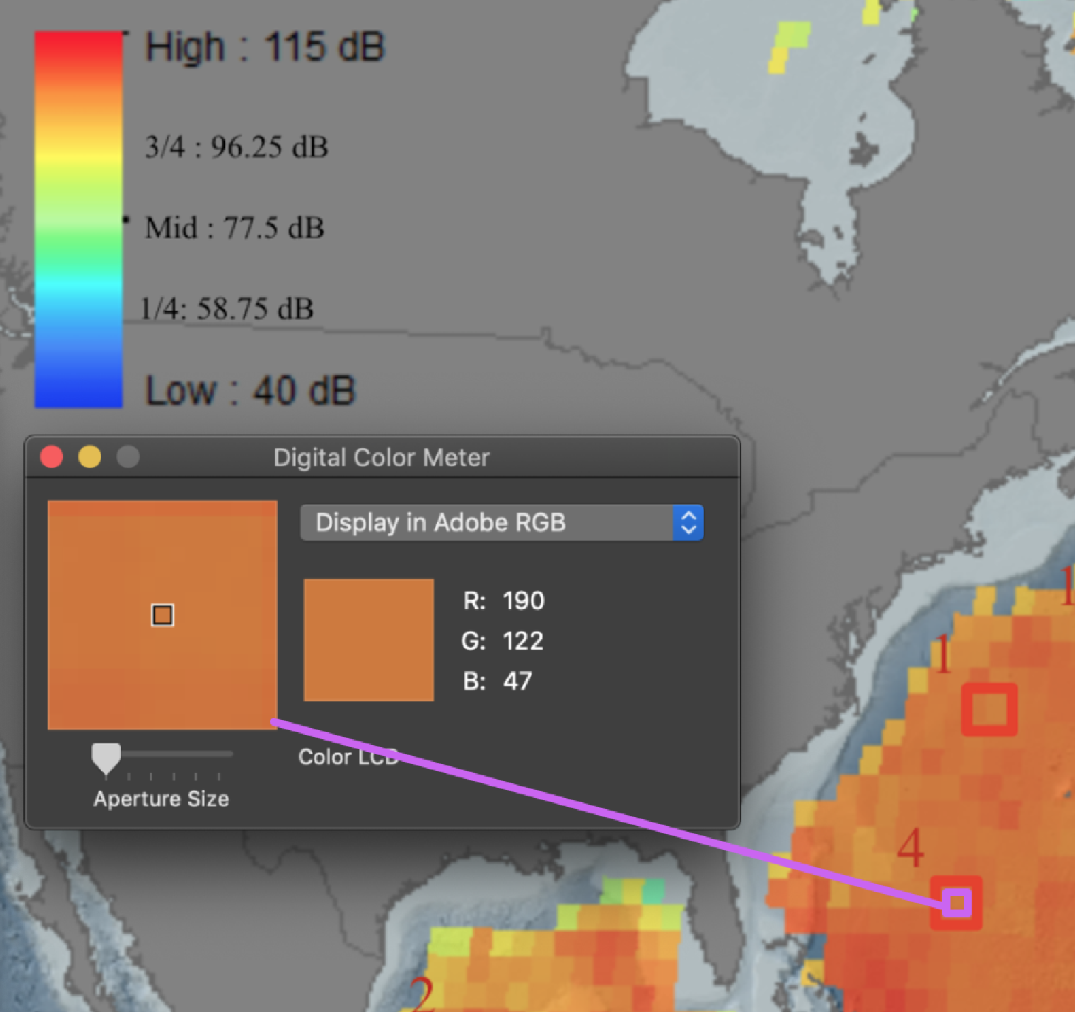
-
Using an Apple computer, use a built-in application, Digital Color Meter, for the observation of values including red green and blue on the screen (Figure 1).
- NOTE: This can be done using other computers, yet it was not used, nor has been tested.
- Pick twenty points at random from the map.
- Number the points on the map 1 through 20.
- Match the value of a point to the red, green, and blue on the scale, as seen in figure 1.
- Record the point number and the decibel figure on the data table.
- Repeat steps five and six for both years.
Part 2
- Obtain shipping route maps from 2002 and 2004 of The Atlantic Ocean, Gulf of Mexico, and Gulf of California.
- Use the legends on the shipping maps to gather data about the points on decibel map. The data should be classified a certain degree based on the level of shipping happening in the area.
- Relate the qualitative data to quantitative data using the following key, Very low – 1, Low – 2, Mid – 3, High – 4, Very High – 5.
- Add the shipping route data to the already existing table that holds the soundscape data from part 1.
- Repeat steps 2 – 4 for both 2002 and 2004.
Ethical Considerations
Considerations of used taken data
- Disturbances to the ecosystems that were tested
- Addition of pollutants in the air from the boat that took the original data.
- Consideration of the energy used
- Additional sound added to the ecosystems being taken
Analyzation of the data
- Consideration of the energy being used in the process of analyzing the data
Results
Figure 2 (Sound in the sea from 2002) [10]
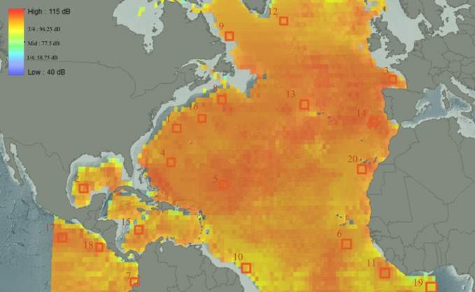
Figure 3 (Sound in the sea from 2004) [11]
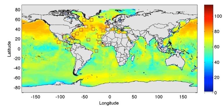
Figure 4 (Shipping routes from 2002)[12]
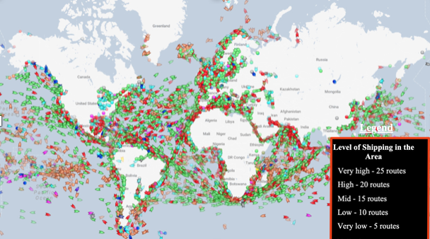
Figure 5 (Shipping routes from 2004) [13]
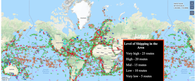
Table 1 Data from 2002
|
Point on the Map |
Decibel level (dB) |
Level of Shipping Happening in the Area (qualitative) |
Level of shipping (quantitative) |
|
1 |
95 |
High |
4 |
|
2 |
66 |
Very low |
1 |
|
3 |
105 |
Very high |
5 |
|
4 |
57 |
Very low |
1 |
|
5 |
97 |
High |
4 |
|
6 |
93 |
Mid |
3 |
|
7 |
92 |
Mid |
3 |
|
8 |
100 |
Very High |
5 |
|
9 |
74 |
Very low |
1 |
|
10 |
77 |
Low |
2 |
|
11 |
79 |
Low |
2 |
|
12 |
84 |
Low |
2 |
|
13 |
95 |
High |
4 |
|
14 |
104 |
Very high |
5 |
|
15 |
62 |
Very low |
1 |
|
16 |
95 |
High |
4 |
|
17 |
61 |
Very low |
1 |
|
18 |
91 |
High |
4 |
|
19 |
94 |
High |
4 |
|
20 |
97 |
Very high |
5 |
Table 2 Data from 2004
|
Point on the Map |
Decibel level (dB) |
Level of Shipping Happening in the Area (qualitative) |
Level of shipping (quantitative) |
|
1 |
112 |
Very high |
5 |
|
2 |
95 |
Low |
2 |
|
3 |
113 |
Very high |
5 |
|
4 |
98 |
Very low |
1 |
|
5 |
111 |
Very high |
5 |
|
6 |
97 |
Mid |
3 |
|
7 |
100 |
High |
4 |
|
8 |
98 |
Mid |
3 |
|
9 |
103 |
Very low |
1 |
|
10 |
100 |
Mid |
3 |
|
11 |
112 |
High |
4 |
|
12 |
99 |
Very low |
1 |
|
13 |
112 |
Very high |
5 |
|
14 |
114 |
Very high |
5 |
|
15 |
99 |
Very low |
1 |
|
16 |
106 |
Very high |
5 |
|
17 |
113 |
Very high |
5 |
|
18 |
110 |
High |
4 |
|
19 |
94 |
Mid |
3 |
|
20 |
93 |
Mid |
3 |
Processed data
The quantitative data in table one and two were derived from the qualitative data, using the following rules.
Very low – 1
Low – 2
Mid – 3
High – 4
Very High – 5
Mean
The mean was taken to provide a concise set of numbers to be referenced to aid in the conclusion. The mean was used for the decibel levels for both years along with the levels of shipping for both years.
Equation for taking the mean:
m = (x1 + x2 + x3 + … + xy) / n
m = mean
y = term number
n = number of terms
x = term
Mean equations for both years of decibel levels:
Mean decibel levels from 2002
m = (95 + 66 + 105+ 57 + 97 + 93 + 92 + 100 + 74 + 77 + 79 + 84 + 95 + 104 + 62 + 95 + 61 + 91 + 94 + 97)
m = 1718 / 20
m = 85.9 dB
Mean decibel levels from 2004
m = (112 + 95 + 113 + 98 + 111 + 97 + 100 + 98 + 103 + 100 + 112 + 99 + 112 + 114 + 99 + 106 + 113 + 110 + 94 + 93)
m = 2064 / 20
m = 103.95 dB
Table 3 Mean Decibel level calculations for both years
|
Year |
Mean decibel levels (dB) |
|
2002 |
85.9 |
|
2004 |
103.95 |
Graph 1 Mean decibel level calculation for the two years
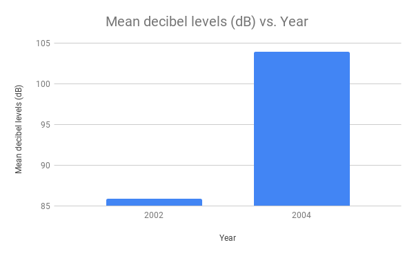
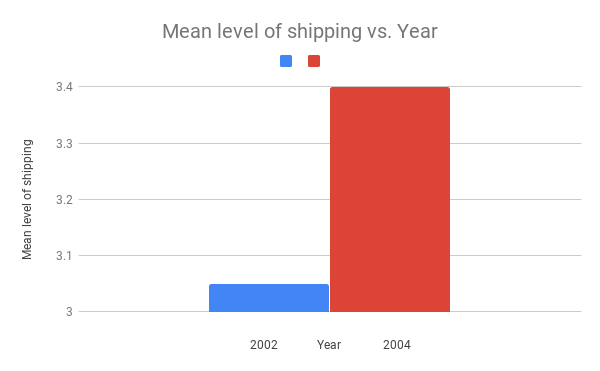
Table 4 Mean levels of shipping for the two years
|
Year |
Mean level of shipping |
|
2002 |
3.05 |
|
2004 |
3.4 |
Graph 2 Mean levels of shipping of 2002 and 2004
Standard deviation
Equation for standard deviation
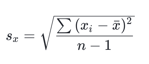
xi = individual values
x̅ = is the mean/expected value
n = the total number of samples
Standard deviation was taken to allow for the understanding of how close the data was to the midpoint.
Table 5 Standard deviation calculations of the mean decibel value
|
Year |
Standard deviation |
|
2002 |
14.97 |
|
2004 |
6.99 |
Table 6 Standard deviation calculations of the shipping levels (quantitative)
|
Year |
Standard deviation |
|
2002 |
1.53 |
|
2004 |
1.54 |
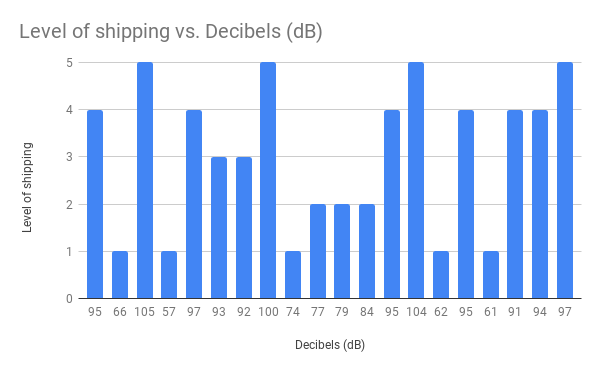
Graph 3 Corresponding severity level vs. Decibels for 2002
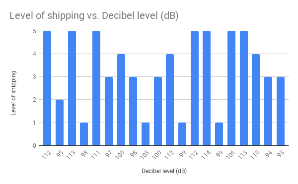
Graph 4 Corresponding severity level vs. Decibels for 2004
Conclusion
The data collected exhibits an answer to the question – to what extent have humans impacted the noise levels (measured in decibels) of the Atlantic Ocean, Gulf of Mexico, and Gulf of California through shipping activity when comparing 2002 to 2004, as measured through the use of hydrophones?
Citing table 5, the standard deviation of the mean decibel levels for 2002 was found to be
14.97 and 2004 to be
6.99. The highest decibel levels recorded in 2004 were along the west coast of Europe and Africa. In addition, the decibel levels of the west coast of Mexico and east coast of Canada aggressively grew between the two years. The least affected areas of the two years include point 2 on the map (Gulf of Mexico), and point 19 (off the east coast of Africa).
When graphing the quantitative value for the level of shipping against the decibel level for both years, graphs 3 and 4, a pattern can be observed, with few exceptions. As decibel levels increase, so does the levels of shipping. The trend can also be observed by looking at the raw data. From 2002 to 2004, the mean level of shipping increased by 0.35, as did the mean sound level in the Atlantic Ocean, Gulf of Mexico, and Gulf of California, increasing by approximately 18.05 decibels, as seen in table 3. Referencing data tables 1 and 2 alongside graph 2, from 2002 to 2004, traffic increased significantly. Thus, showing that as one variable increases (shipping), so does the other (decibel levels).
Discussion
The span of the two years examined had a large effect on the soundscape in the Atlantic Ocean. This can be attributed to the increase in shipping off the coasts of North America, South America, Africa, and Europe. The increase of ship traffic at sea has subsequently led to an increase in underwater noise levels. Shown by graphs 3 and 4, there is direct correlation, with scarce outliers.
A possible reason for the increase may be more frequent transportation of supplies around the world. During the span of 1980 to 2018, container ship capacity grew, starting at about 11 million metric tons to around 253 million metric tons[14], while the number of ships at sea also grew[15]. To accommodate the increase in shipping, logically new ports would have opened, in addition to the size of many ports increasing between the two years. Predicting for the future, based on the current trend, the volume being shipped across the Atlantic Ocean, Gulf of Mexico, and Gulf of California will increase. Consequently, the number of ships will also increase, leading to the creation of an even louder soundscape.
With underwater noise levels increasing, cetaceans trying to find mates, feed, navigate, and keep track of their young are at a disadvantage. A large concern is that even a slender increase in decibels may make these practices more difficult than they already are[16]. Comparing graphs 3 and 4 indicates that cetaceans that would have communicated in 2002, had a different experience than their counterparts in 2004 due to the decreased distance that their communications could reach as a result of human interference.
Evaluation
The original concept of analyzing soundscape maps of the Tasman Sea was limited by the absence of soundscape maps available to the general public. The absence is predicted to be filled as soundscape maps continue to be constructed and distributed. Thus, a wider selection will eventually be available allowing for the analyzation of more remote parts of the world.
A clear and resourceful approach to analyzing data was taken, allowing for a precise reading of maps to be recorded in the data tables. The reinforcement of rational data allowed for a clearer answer to the research question. Assigning severity levels was challenging when attempting to quantify the data of the shipping route maps. Various other methods of quantifying data could lead to an improved set of data points of which conclusions could be extracted. Another challenge arose when picking points on the soundscape maps to analyze.
Modifications for the future
Measuring the soundscape at more points to try and achieve a clearer understanding. Instead of randomly picking points, other methods could be utilized in hopes of displaying more trends, such as solely testing on the coasts of continents. Looking into cetacean migration patterns in the tested areas of the ocean to allow for a more in-depth answer to the research question. This could be completed by using two maps of the soundscape of a specific year, but in different seasons, alongside two maps of shipping routes of the same year in different seasons to try and account for the migration patterns.
Solutions
NOAA is leading the way in setting up and maintaining a network of acoustic monitoring devices that would set a strong foundation for any actions going forward[17]. The knowledge and understanding of the severity of past human actions would allow us to move forward with a more informed view of the consequences that follow. These technologies would aid in continuous monitoring of the underwater soundscapes with greater certainty and higher efficiency. As mentioned in the Evaluation, the sparse number of soundscape maps available to the public hinder the analyzing that third parties could accomplish. The increased production would allow for more groups to measure soundscapes. Yet, with a larger production of hydrophones also comes the addition of harmful chemicals in the air (leading to acid deposition), the creation of sound pollution from transporting said materials, use of energy throughout the whole process, and further environmental impacts. The endeavor of engineering noise-reduction technologies that would be affixed to ships is underway[18]. The addition of noise reducing technologies on ships would assist in the lowering of the soundscape decibel levels, while still allowing humans to ship goods across vast bodies of water.
Going further with research
How might the soundscape be different at varying depths? How do local communities interact with the increase of decibels? How quickly might areas recover from the withdrawal of the high levels of decibels? Have cetaceans evolved new approaches to combat the rising decibel levels? Are cetaceans migrating to different parts of the world as a result of the rising decibel levels? How do shipping levels vary from season to season?
Word count: Approx. 2100 (not including the bibliography nor footnotes, nor data)
References
- Au, Whitlow W. L., and James A. Simmons. “Echolocation in Dolphins and Bats.” Physics Today, American Institute of Physics, 1 Sept. 2007, physicstoday.scitation.org/doi/10.1063/1.2784683.
- National Marine Mammal Laboratory. “National Marine Mammal Laboratory.” Marine Mammal Education Web, NOAA, 21 Aug. 2006, www.afsc.noaa.gov/nmml/education/cetaceans/cetaceaechol.php.
- “The Evolution of Whales.” Reproductive Isolation, evolution.berkeley.edu/evolibrary/article/evograms_03.
- Milman, Oliver. “Ships’ Noise Is Serious Problem for Killer Whales and Dolphins, Report Finds.” The Guardian, Guardian News and Media, 2 Feb. 2016, www.theguardian.com/environment/2016/feb/02/ships-noise-is-serious-problem-for-killer-whales-and-dolphins-report-finds.
- US Department of Commerce, and National Oceanic and Atmospheric Administration. “Listen Up: What You Need to Know About Ocean Noise.” NOAA’s National Ocean Service, 29 Aug. 2018, oceanservice.noaa.gov/podcast/aug18/nop18-ocean-noise.html.
- National Marine Mammal Laboratory. “National Marine Mammal Laboratory.” Marine Mammal Education Web, NOAA, 21 Aug. 2006, www.afsc.noaa.gov/nmml/education/cetaceans/cetaceaechol.php.
- Rice, Catherine. “Humans Are Changing the Underwater Soundscapes of the World’s Oceans.” Nature World News, 13 June 2017, www.natureworldnews.com/articles/38419/20170613/humans-changing-underwater-soundscapes-oceans.htm.
- “Global Merchant Fleet – Number of Ships by Type 2017 | Statistic.” Statista, www.statista.com/statistics/264024/number-of-merchant-ships-worldwide-by-type/.
- “Echolocation: Bats and Whales Behave in Surprisingly Similar Ways.” Echolocation: Bats and Whales Behave in Surprisingly Similar Ways, ScienceDaily / University of Southern Denmark, 29 Oct. 2013, www.sciencedaily.com/releases/2013/10/131029101617.htm.
- “Sound Field Data Availability.” Roadmap, cetsound.noaa.gov/sound_data.
- Michael B. Porter and Laurel J. Henderson. “Soundscapes.” Soundscapes, www.onr.navy.mil/reports/FY13/mbporter.pdf.
- MarineTraffic: Global Ship Tracking Intelligence | AIS Marine Traffic, www.marinetraffic.com/en/ais/home/centerx:39.7/centery:44.1/zoom:2.
- MarineTraffic: Global Ship Tracking Intelligence | AIS Marine Traffic, www.marinetraffic.com/en/ais/home/centerx:39.7/centery:44.1/zoom:2.
- Laporte, John. “Topic: Container Shipping.” Statista, www.statista.com/topics/1367/container-shipping/.
- Tournadre, Jean. “Worldwide Ship Traffic up 300 Percent since 1992.” “Anthropogenic Pressure on the Open Ocean: the Growth of Ship Traffic Revealed by Altimeter Data Analysis,” AGU, news.agu.org/press-release/worldwide-ship-traffic-up-300-percent-since-1992/.
- Milman, Oliver. “Ships’ Noise Is Serious Problem for Killer Whales and Dolphins, Report Finds.” The Guardian, Guardian News and Media, 2 Feb. 2016, www.theguardian.com/environment/2016/feb/02/ships-noise-is-serious-problem-for-killer-whales-and-dolphins-report-finds.
- “Phase 2 — NOAA’s Ocean Noise Strategy.” Cetacean & Sound Mapping, NOAA, cetsound.noaa.gov/ons.
- Raymond Fischer and Kurt Yankaskas. Noise Control on Ships – Enabling Technologies. apps.dtic.mil/dtic/tr/fulltext/u2/a553403.pdf.
[1] Au, Whitlow W. L., and James A. Simmons. “Echolocation in Dolphins and Bats.” Physics Today, American Institute of Physics, 1 Sept. 2007, physicstoday.scitation.org/doi/10.1063/1.2784683.
[2] National Marine Mammal Laboratory. “National Marine Mammal Laboratory.” Marine Mammal Education Web, NOAA, 21 Aug. 2006, www.afsc.noaa.gov/nmml/education/cetaceans/cetaceaechol.php.
[3] “The Evolution of Whales.” Reproductive Isolation, evolution.berkeley.edu/evolibrary/article/evograms_03.
[4] Milman, Oliver. “Ships’ Noise Is Serious Problem for Killer Whales and Dolphins, Report Finds.” The Guardian, Guardian News and Media, 2 Feb. 2016, www.theguardian.com/environment/2016/feb/02/ships-noise-is-serious-problem-for-killer-whales-and-dolphins-report-finds.
[5] US Department of Commerce, and National Oceanic and Atmospheric Administration. “Listen Up: What You Need to Know About Ocean Noise.” NOAA’s National Ocean Service, 29 Aug. 2018, oceanservice.noaa.gov/podcast/aug18/nop18-ocean-noise.html.
[6] National Marine Mammal Laboratory. “National Marine Mammal Laboratory.” Marine Mammal Education Web, NOAA, 21 Aug. 2006, www.afsc.noaa.gov/nmml/education/cetaceans/cetaceaechol.php.
[7]Rice, Catherine. “Humans Are Changing the Underwater Soundscapes of the World’s Oceans.” Nature World News, 13 June 2017, www.natureworldnews.com/articles/38419/20170613/humans-changing-underwater-soundscapes-oceans.htm.
[8] “Global Merchant Fleet – Number of Ships by Type 2017 | Statistic.” Statista, www.statista.com/statistics/264024/number-of-merchant-ships-worldwide-by-type/.
[9]“Echolocation: Bats and Whales Behave in Surprisingly Similar Ways.” Echolocation: Bats and Whales Behave in Surprisingly Similar Ways, ScienceDaily / University of Southern Denmark, 29 Oct. 2013, www.sciencedaily.com/releases/2013/10/131029101617.htm.
[10] “Sound Field Data Availability.” Roadmap, cetsound.noaa.gov/sound_data.
[11] Michael B. Porter and Laurel J. Henderson. “Soundscapes.” Soundscapes, www.onr.navy.mil/reports/FY13/mbporter.pdf.
[12]MarineTraffic: Global Ship Tracking Intelligence | AIS Marine Traffic, www.marinetraffic.com/en/ais/home/centerx:39.7/centery:44.1/zoom:2.
[13] MarineTraffic: Global Ship Tracking Intelligence | AIS Marine Traffic, www.marinetraffic.com/en/ais/home/centerx:39.7/centery:44.1/zoom:2.
[14] Laporte, John. “Topic: Container Shipping.” Statista, www.statista.com/topics/1367/container-shipping/.
[15] Tournadre, Jean. “Worldwide Ship Traffic up 300 Percent since 1992.” “Anthropogenic Pressure on the Open Ocean: the Growth of Ship Traffic Revealed by Altimeter Data Analysis,” AGU, news.agu.org/press-release/worldwide-ship-traffic-up-300-percent-since-1992/.
[16] Milman, Oliver. “Ships’ Noise Is Serious Problem for Killer Whales and Dolphins, Report Finds.” The Guardian, Guardian News and Media, 2 Feb. 2016, www.theguardian.com/environment/2016/feb/02/ships-noise-is-serious-problem-for-killer-whales-and-dolphins-report-finds.
[17] “Phase 2 — NOAA’s Ocean Noise Strategy.” Cetacean & Sound Mapping, NOAA, cetsound.noaa.gov/ons.
[18] Raymond Fischer and Kurt Yankaskas. Noise Control on Ships – Enabling Technologies. apps.dtic.mil/dtic/tr/fulltext/u2/a553403.pdf.
Cite This Work
To export a reference to this article please select a referencing stye below:
Related Services
View all


DMCA / Removal Request
If you are the original writer of this essay and no longer wish to have your work published on UKEssays.com then please click the following link to email our support team:
Request essay removal