Warrington Environmental Pollution and Soil Health Risks

Report on the environmental pollution and human health risks of soils in the former industrial area of Woolston, Warrington.

2.Introduction:

As a result of rapid population growth followed by intense industrial activity and petrochemical development soils have suffered from contamination with substances of various origins (E.M.Garcia et al,2015).As a result of rapid industrialisation of cities such as Manchester, newly constructed canals were built all over the UK in order to increase trade as well as the exportation of goods. In the 1820’s, a new canal was established along the river Mersey with the purpose of shortening the route of navigation through the meandering Mersey.

3.Study site.

According to Warrington borough council, the New Cut Canal was opened in 1821. This 2km long canal was built in order to improve the Mersey and Irwell navigation by creating a shortcut for barges carrying goods between Liverpool and Manchester. Historical ordnance survey maps from 1907 show an adjacent chemical works, a large tannery, a slaughter house, a metal works and a gunpowder mill. Sustained industrial activity meant that the canal sediment was undoubtedly polluted by spillages from ships and industrial effluents (Hartley and Dickinson,2010). Following the establishment of the Manchester shipping canal the New Cut Canal began to decline until it was left derelict (Warrington borough council) and eventually the Canal was disconnected from the river and abandoned in 1978 (Hartley and Dickinson,2010). In that year, it was decided that the site was to be used for tipping under emergency procedures to deposit road construction rubble (Hartley and Dickinson ,2010).

Following this history, it has been estimated that the site contains 9800 tonnes of polluted anoxic sediment. It is known that this polluted sediment contains elevated levels of TPH’s (Total Petroleum Hydrocarbons), PAH’s (Polycyclic Aromatic Hydrocarbons) followed by highly elevated concentrations of metals (Pb, Zn, Cu, Cr and Ni) and Arsenic (As) (Hartley and Dickinson,2010).

4.Methods:

4.1. Methods out in the field.

4.1.1 Soil samples

To determine the degree of soil contamination at the site, soil samples were taken at various points along the New Cut Canal site. It was decided that a systematic sampling method would be used in order to record an adequate amount of data for the investigation. This sampling method had been chosen as it allowed one to determine the spatial pattern of contamination whilst limiting human errors (O1). Whilst at the site, transects had been established along the New Cut Canal site. Transects were established along a 700-metre stretch of the canal and each transect had been separated by 70 meters. In total there was 10 transects and along each transect,6 soil samples were taken approximately every 10 meters from the Northernmost point of the canal to the southernmost point closest to the river Mersey.

Soil samples from each sampling point were taken just below the surface but in order to prevent large organic materials from interfering with the soil investigations later it was decided that each sample should be taken and the large organic matter (Roots etc.) should be removed. This was done using a measuring tape and a spade. The soil samples had been gathered in plastic bags.

4.2. Conductivity and resistivity values within the soil surrounding New Cut Canal.

4.2.1. Electrical Resistivity Imaging (ERI) using ERT (Electrical Resistivity Tomography)

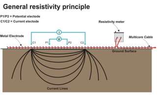
The ERI was used to show the potential mobility of trace and toxic metals within the soil by analysing conductivity data from the ERT and the EM-31. Conductivity measurements were taken using an ERT along a single transect measuring 35 metres between the New Cut Canal site and the river Mersey. The ERT takes conductivity measurements through a series of electrodes which are placed into the ground. Once these electrodes had been implanted and connected to each other via multi core cables a current was then injected into the ground through these electrodes and as the current passed through the soil resistivity measurements were taken. Changes in conductivity reflect variations in subsurface materials and higher conductivity readings are associated with higher metal concentrations in soil pore waters.

Figure 1: Below is an image that shows the standard setup of ERT. In this investigation the electrodes were inserted into the ground at distances of 2 meters apart. The transect of electrodes covered an area between the New Cut Canal and the river Mersey and was carried out at an angle of 0^° (North to South). Image from Terra Dat:  http://terradat.co.uk/survey-methods/resistivity-tomography/

4.2.2. Geonics EM-31 Ground Conductivity meter

ERT maps out the geological variations associated with changes in conductivity (Exploration instruments) as well as the EM-31. Unlike the ERT, the EM-31 gathers its readings by creating an electromagnetic field in the air using a coil wire which is separated from a receiver coil by 3.66 meters. The transmitted energy propagates into the subsurface where a second electromagnetic field is created due to the effect of soil moisture, conductive earth materials and other buried objects (Reynolds international,2011). The EM-31 is useful to this investigation as it can take conductivity measurements below 2 meters of the Earth’s surface. The data collected by both the EM-31 and the ERT could then be combined to determine changes in conductivity up to a depth of 3-4 meters.

4.3. Soil sample experiments in the lab

4.3.1. Determining total metal concentrations

Following the onsite extraction of soils samples, they were then taken to the lab for further processing. Before any more investigations were conducted the soil samples were dried in an oven at 40°C for 48 hours in order to remove all of the moisture.  Oven drying the sediment is crucial in this type of investigation as one can only compare the dry weight to the Soil Guideline Values (SGV’s) (DEFRA, 2002). Once they had been dried, the soil samples were then processed further in order to analyse the total metal concentrations (Pb,Zn,Cr and As), bioavailability of those metals, organic matter content and soil pH. Soil samples were then sieved so that larger particles greater than 2mm in diameter were removed.  After the samples had been sieved, analysis of the bioavailability of metals was conducted. 10g of sieved sediment was then added to a conical where 50mL of 0.5mol acetic acid was added using a measuring cylinder. Once the acid was added the flask was sealed with Parafilm and placed onto an orbital shaker for 30 minutes. Whilst the samples were shaken, 2 30mL universal sample tubes were prepped (2 for every sample) and a Whatman no 1 filter paper was added to each of the tubes. After the cylinder samples had been shaken, they were left to stand for 10 minutes in order for the contents to settle (Beneficial to the investigation as it sped up the filtering process). Following 10 minutes, the supernatant liquid in the cylinder was then added into the universal sample tubes through the filter paper. Once one of the tubes was full the second one was then introduced to the filtering process. Eventually both universal tubes were sealed and then analysis of the metal concentrations was conducted by Atomic Absorption Spectroscopy (AAS).

4.3.2. Determining organic matter (OM) content

Secondly, organic matter content needed to be measured, this was done using the loss on ignition method. This process began with the weighing of an empty porcelain crucible (W1). Soil was then added until it filled the crucible and was then weighed (W2). The air-dry weight was then determined by using the following calculation W2-W1. The minute that this was done the crucibles for each of the samples was then oven-dried at a temperature of 105°C overnight and then placed in a desiccator the following morning. Afterwards, the samples were then measured again (W3). The crucibles were then placed into a muffle furnace and ignited at 450°C for 8 hours and left to cool on a sand tray. After this, the crucibles were weighed again (W4). This was done to burn off any of the Organic Matter (OM) content. Muffled weight was then determined by using this calculation, W4-W1. The final method involved a simple calculation, shown below:

OM content (% of dry sediment) =

[oven dry weight (g) – muffled weight (g) / oven dry weight (g)] x 100

4.3.3. Determining soil pH

To begin with 10g of soil was added to a beaker using a spatula where it would then be mixed with 25mL of deionised water using a measuring cylinder. The beaker was then stirred well until all of the material had been suspended (To allow the contents to mix) shortly followed by a 15-minute period whereby the beaker was left to stand. Following the 15-minute period a pH strip was dipped into each of the samples. Using a pH reference card, the colours recorded on each of the pH papers was noted.

4.3.4. Determining Total (T) metal concentrations using XRF (X-Ray Fluorescence Spectroscopy)

Finally, 10g of each sample was added into a small plastic bag and then shaken until all of the soil reached the bottom. The bag was then placed onto the test bed and then the XRF machine determined the % values of Pb, Zn, Cr and As.

5. Results

5.1.

Figure 2: The table below shows all of the data collected from the field as well as metal concentrations in mg/kg^-1 for each of the soils samples. OM or organic matter was measured in grams. Total Chromium concentrations when analysed however the concentrations were too low when measured using X-Ray Fluorescence Spectroscopy (XRF).

Figure 3: The image below shows the spatial pattern of Lead (Pb) contamination across the New Cut Canal site. The image was created using Arc Map software. It is clear that the highest levels of Pb were found around sample site A3-5 and H1-2.

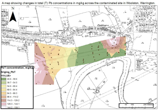
Figure 4: The image below shows the spatial pattern of Zinc (Zn) contamination across the New Cut Canal site. The image was created using Arc Map software. Based on the spatial image, it is clear that the highest levels of Zn were found around sampling sites H1 and H2.

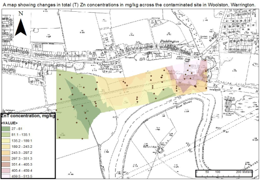
Figure 5: The image below shows the spatial pattern of pH levels across the New Cut Canal site. The image was created using Arc Map. The most acidic pH readings were located towards the Southwest of the site whereas pH readings in the Eastern part of the sampling site increased to a pH of 5.3 and above.

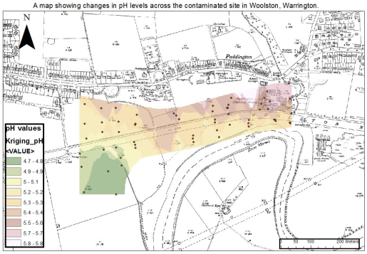
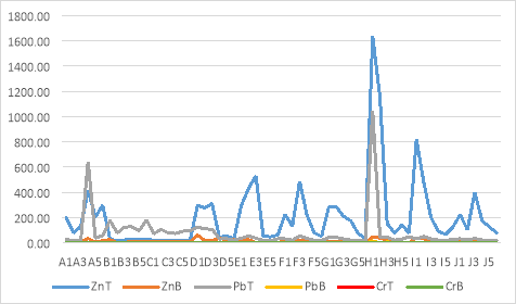Figure 6: The graph below represents the changes in the Total (T) metal concentrations of various metals as well as indicating how bio available these metals are in the area.

Figure 7: The stacked column below allows one to determine the bioavailability of Zinc as a percentage when compared to its total (T) metal concentrations for each of the sample sites. Upon observing the data, it is clear that (in terms of percentage) Zn bioav