Viscoplasticity and Static Strain Ageing

Viscoplasticity

Inelastic deformation of materials is broadly classified into rate independent plasticity and rate dependent plasticity. The theory of Viscoplasticity describes inelastic deformation of materials depending on time i.e. the rate at which the load is applied. In metals and alloys, the mechanism of viscoplasticity is usually shown by the movement of dislocations in grain [21]. From experiments, it has been established that most metals have tendency to exhibit viscoplastic behaviour at high temperatures. Some alloys are found to exhibit this behaviour even at room temperature. Formulating the constitutive laws for viscoplasticity can be classified into the physical approach and the phenomenological approach [23]. The physical approach relies on the movement of dislocations in crystal lattice to model the plasticity.   In the phenomenological approach, the material is considered as a continuum. And thus  the microscopic behaviour can be represented by the evolution of certain internal variables instead. Most models employ the kinematic hardening and isotropic hardening variables in this respect. Such a phenomenological approach is used in this work too.

According to the classical theory of plasticity, the deviatoric stresses is the main contribu- tor to the yielding of materials and the volumetric or hydrostatic stress does not influence the inelastic behaviour. It also introduces a yield surface to differentiate the elastic and plastic domains. The size and position of such a yield surface can be changed by the strain history, to model the exact stress state. The theory of viscoplasticity differs from the plasticity theory, by employing a series of equipotential surfaces. This helps define an over-stress beyond the yield surface. The plastic strain rate is given by the viscoplastic flow rule. To model the hardening behaviour, introduction of several internal variables is necessary. Unlike strain or temperature which can be measured to asses the stress state, internal variable or state variables are used to capture the material memory by means of evolution equations. This must include a tensor variable to define the kinematic hardening and a scalar variable to define the isotropic variable. The evolution of these internal variables allows us to define the complete hardening behaviour of materials. In this work we consider only the small strain framework.

The basic principles of viscoplasticity are similar to those from Plasticity theory. The main difference is the introduction of time effects. Thus the concepts from plasticity and the introduction of time effects to describe viscoplasticity, as summarised by Chabocheand Lemaitre[21] are discussed in this chapter.

1. Basic principles

Considering small strains framework, the strain tensor can be split into its elastic and inelastic parts

ε = εe+ εin(2.1)

where ε is total strain, εe is the elastic strain and εin is the inelastic strain. In this work, we neglect creep and thus consider only the plastic strain to be the inelastic strain. Hence we can proceed to rewrite the above equation as :

ε = εe+ εp(2.2)

where εp is the plastic strain. Let us consider a field with stress σ = σi j(x) and external volume forces fi. Thus the equilibrium condition is given as:

∂σi j + f

∂xii

= 0;i, jε

{1,2,3}

(2.3)

From the balance of moment of momentum equation, we know that the Cauchy stress ten- sor is symmetric in nature. The strain tensor is calculated from the gradient of displacement, uas:

1 .∂uj∂ui.

εi j = 2

∂xi

+ ∂x

(2.4)

The Hooke’s law for the relation between stress and strain tensors is given using the elastic part of the strain:

σ = E· εe(2.5)

where εe and the stress σ are second order tensors. E is the fourth order elasticity tensor.

2. Equipotential surfaces

In the traditional plasticity theory which is time independent, the stress state is governed by a yield surface and loading-unloading conditions. In Viscoplasticity the time or rate dependent plasticity is described by a series of concentric equipotential surfaces. The location on the centre and its size determine the stress state of a given material.

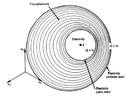
Fig. 2.1 Illustration of equipotential surfaces from [21]

It can be understood that the inner most surface or the surface closest to the centre represents a null flow rate(Ω = 0). As shown in Figure (2.1), the outer most and the farthest surface from the centre represents infinite flow rate (Ω = ∞). These two surfaces represent the extremes governed by the time independent plasticity laws. The region in between is governed by Viscoplasticity[21]. The size of the equipotential surface is proportional to the flow rate. Greater the flow, greater is the surface size. The region between the centre and the inner most surface is the elastic domain. Flow begins at this inner most surface( f=0).

In Viscoplasticity, there are two types of hardening rules to be considered: (i) Kinematic hardening and (ii) isotropic hardening. The Kinematic hardening describes the movement of the equipotential surfaces in the stress plane. From material science, this behaviour is known to be the result of dislocations accumulating at the barriers. Thus it helps in describing the Bauschinger effect [27] which states that when a material is subjected to yielding by    a compressive load, the elastic domain is increased for the consecutive tensile load. This behaviour is represented by α which does not evolve continuously during cyclic loads and thus fails to describe cyclic hardening or softening behaviours. A schematic representation is shown in Fig.(2.2).

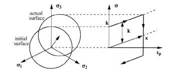
Fig. 2.2 Linear Kinematic hardening and Stress-strain response from [11]

The isotropic hardening on the other hand describes the change in size of the surface and assumes that the centre and shape remains unchanged. This behaviour is due to the number of dislocations in a material and the energy stored in it. It is represented by variable r, which evolves continuously during cyclic loadings. This can be controlled by the recovery phase. As a result, isotropic behaviour is helpful is modelling the cyclic hardening and softening phenomena. A schematic representation is shown in Fig.(2.3).

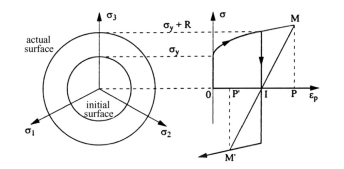
Fig. 2.3 Linear Isotropic hardening and Stress-strain response from [11]

From Thermodynamics, we know the free energy potential(ψ ) to be a scalar function [21]. With respect to temperature T, it is concave. But convex with respect to other internal variables. Thus, it can be defined as :

ψ= ψ.  ,T,εe,εp,Vk.(2.6)

where ε,Tare the only measured quantities that can help model plasticity. Vkrepresents the set of internal variable, also known as state variables which help define the memory of the previous stress states.

In Viscoplasticity, it is assumed that ψ depends only on εe,T,Vk. Thus we have:

ψ= ψ.  e,T,Vk.(2.7)

According to thermodynamic rules, stress is associated with strain and the entropy with temperature. This helps us define the following relations:

σ = ρ

. ∂ψ.

∂εe

,s = −

.∂ψ.

∂T

(2.8)

where ρ is density and s is entropy. It is possible to decouple the free energy function and split it into the elastic and plastic parts.

ψ= ψe.  e,T.+ ψp.  ,r,T.(2.9) Similar to σ, the thermodynamic forces corresponding to α and r is given by:

X = ρ

.∂ψ.

∂α

,R = ρ

.∂ψ.

∂r

(2.10)

Here we have X the back stress tensor, used to measure Kinematic hardening. It is noted as a Kinematic hardening variable which defines the position tensor of the centre of equipotential surface. Similarly Ris the Isotropic hardening variable which governs the size of the equipotential surface.

3. Dissipation potential

The equipotential surfaces that describe Viscoplasticity have some properties.

• Points on each surface have a magnitude equal to the strain rate.

• Points on each surface have the same dissipation potential.

• If potential is zero, there is no plasticity and it refers to the elastic domain.

The dissipation potential is represented by Ω which is a convex function. It can be defined in a dual form as:

Ω = Ω.  ,X,R; T,α,r.(2.11)

It is a positive function and if the variables σ,X,Rare zero, then the potential is also zero. The normalityrule, defined in [22] suggests that the outward normal vector is proportional to the gradient of the yield function. Applying the normality rule, we may obtain the following relations:

∂Ω εË™  p = ∂σ,

αË™  = ∂Ω ,

∂X

∂ Ω

rË™ =

∂R

(2.12)

Considering the recovery effects in Viscoplasticity, the dissipation potential can be split into two parts:

Ω = Ωp+ Ωr(2.13)

where Ωp is the Viscoplastic potential and Ωr  the recovery potential which are defined as :

Ωp=Ωp..− X. − R− k,X,R; T,α,r. ,(2.14)

Ωr=Ωr.  ,R; T,α,r.(2.15)

.3

J2 .

. ′′.′′

σ− X=2   σ− X:   σ − X

(2.16)

where J2 .− X. refers to the norm on the stress plane and kis the initial yield or the initial

size of equipotential surface.

Going back to the relation in (2.12) , we have:

∂J2 .

• X.

σ′ − X ′

σ

∂Ω∂Ω

εË™         ==

3

=pË™

(2.17)

p∂σ∂J2 .

.∂σ

2σ− X.

Here, p is the accumulated viscoplastic strain, given by :

.2

pË™   =

εË™  p : εË™p(2.18)

3

Also applying the normality rule on eq. (2.15) we may define r as :

rË™ = pË™ −

∂Ωr(2.19)

∂R

Thus when recovery is ignored (i.e Ωr = 0), r is equal to p.

4. Perfect viscoplasticity

Let us consider pure viscoplasticity where hardening is ignored. Thus the internal variables may also be removed.

Ω = Ω. ,T.(2.20)

Since plasticity is independent of volumetric stress, we may consider just the deviatoric stress σ ′ = σ − 1 tr(σ)I. Using isotropic property, we may just use the second invariant of

σ ′. Thus:

Ω = Ω. (σ ),T.(2.21)

Applying the normality rule here, we may obtain the flow rule for Viscoplasticity.

∂Ω3∂Ωσ′

εË™         ==

(2.22)

p∂σ

2 ∂J2 .σ.

J2 .σ.

From the Odqvist’s law [12], the dissipation potential for perfect viscoplasticity can be obtained. Here the elastic part is ignored. Thus we have:

λ

Ω =

n + 1

.J2(σ).n+1

λ

(2.23)

where λ and n are material parameters.

Using this relation in the flow rule from eq.(2.22), we get:

.J2(σ).nσ′

3

εË™          =

p2λ

J2 . .

(2.24)

Further the elasticity domain can be included through the parameter kwhich is a measure of the initial yield:

3

εË™          =

.J2(σ) − k.nσ′

(2.25)

p2λ

J2 . .

The <> are the Macauley brackets defined by :

⟨F⟩ = F· H(F),H(F) =

.1  ifF0

(2.26)

0  ifF <0

5. Hardening rules

As suggested in previous sections, the Viscoplasticity can be enhanced by including internal variables, which help describe the material memory dependent behaviours. These internal variables or state variables include Kinematic and isotropic hardening. Kinematic hardening can help describe the stress hysteresis loops accurately. It governs the movement of the centre of equipotential surfaces and thus the surface by itself. Isotropic hardening helps describe the cyclic hardening and softening effects. It governs the changes in size of the surface.

We have already discussed the normality rule in (2.10), where a relation is  established.

Ignoring the recovery, we have:

X = ρ

.∂ψ.

∂α

,  R = ρ

.∂ψ.

∂r

.∂ψ.

= ρ∂p

(2.27)

Thus the dissipation potential can be written as:

Ω = Ω.σ,X,R; T,α,p.(2.28)

2.2 Static strain ageing11

As suggested in [21], by including αand pin the free energy function and the dissipation potential, the following forms are achieved:

1

ρψ = ρψe + 3 c α : α+ h(p)(2.29)

Ω  = Ω

J2 .

− X. − R− k+ 1

J2(X) − 2

.

c γ J2(α) ; T, p

(2.30)

σ2 c  292 

where k, c, γ are temperature dependent material parameters. From (2.27) and (2.29) the hardening variables can be derived as:

2

X=c α,  R = ρ

3

.∂ψ.

∂ p

(2.31)

Applying the normality rule on (2.29),(2.30) we may get the following terms:

σ′ − X ′

εË™  p = ∂Ω= 3∂Ω

(2.32)

∂σ2 ∂J2 .− X.

..

J2    σ − X

∂ Ω

pË™    = − ∂R=

∂ Ω

.

εË™ p

3

p3

: εË™ p

γ

(2.33)

αË™  = − ∂R= εË™

X pË™

2 c

(2.34)

Substituting the above in (2.31), we obtain the final relations for Kinematic hardening variable and the Isotropic hardening variable as:

XË™      = 2 cεË™pγXpË™ 3

RË™   =b (Q − R) pË™

(2.35)

(2.36)

where b,Qare material parameters. Superposing the kinematic and isotropic hardening rules, a unified Visoplastic model was formulated by Chaboche. An extension of such a model will be used in this work.

2. Static strain ageing

Strain ageing is defined as the rise in material strength and decrease of ductility in a material when heat treated at a low temperature post the cold working[3]. It can be broadly classified into:

• Static strain ageing – If the change in material properties occurs post the ageing period.
• Dynamic strain ageing – If the change in material properties during the ageing period.

Experimental results of low carbon steel specimen subjected to tensile strain and then rested for period of time reveal interesting behaviour. A steel specimen is loaded beyond the yield point and after the hardening has evolved, it is unloaded and rested at 200c for a period of time. On applying the load again, a considerable rise in the yield point is noticed. This phenomenon is termed as Strain ageing. Higher temperatures have been observed to accelerate the ageing. Composition of a material is also known to be a factor.

1. Theory of deformation

A detailed account found in [3] has been summarised here. Metals at a crystal structural level consist of atoms arranged together in patterns which are governed by various factors such as atomic size, temperature and the alloyed elements. Atoms are arranged in layers at different orientations. When enough force is applied on the crystals in certain favourable orientations, the layers of atoms may slip above one another. This phenomena is termed as slip. This slip happens due to the movement of defects or dislocations in the crystal lattice. Depending on the material’s resistance to the slip phenomena, its material properties may be defined. If the slip occurs with less amount of force, then it results in a low yield point during a tensile load. Subsequently the material doesn’t show much hardening behaviour and fractures may occur with a marginal increase in force. This kind of fracture is characterised by good ductility. If a large force is needed to cause this slip, then the material has a high yield point. Material hardening behaviour is also greater. Also greater amount becomes necessary to continue the deformation and cause fracture. This fracture is characterised by poor ductility.

2. Metallurgical causes

Alloys may consist of varying alloying elements in addition to iron. These elements upon cooling, move through the dislocations due to the distortion they create in a crystal lattice. They concentrate arou