Supervised Image Classification Techniques

Introduction

In this chapter, a review of Web-Based GIS Technology and Satellite image classification techniques. Section 2.2 presents a review of Web-Based GIS Technology.in section 2.3 Satellite images classification techniques are reviewed.
In section 2.4 presents the related work .section 2.5 presents uses of web based GIS applications in real world. Section 2.6 presents available commercial web GIS sites. Section 2.7 reviews the types of Geospatial Web Services (OGC)

2.3 Image Classification

Image classification is a procedure to automatically categorize all pixels in an Image of a terrain into land cover classes. Normally, multispectral data are used to Perform the classification of the spectral pattern present within the data for each pixel is used as the numerical basis for categorization. This concept is dealt under the Broad subject, namely, Pattern Recognition. Spectral pattern recognition refers to the Family of classification procedures that utilizes this pixel-by-pixel spectral information as the basis for automated land cover classification. Spatial pattern recognition involves the categorization of image pixels on the basis of the spatial relationship with pixels surrounding them. Image classification techniques are grouped into two types, namely supervised and unsupervised[1]. The classification process may also include features, Such as, land surface elevation and the soil type that are not derived from the image. Two categories of classification are contained different types of techniques can be seen in fig

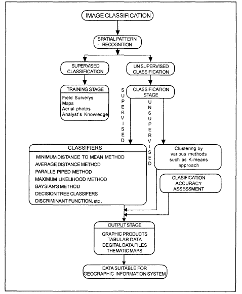
Fig. 1 Flow Chart showing Image Classification[1]

2.3 Basic steps to apply Supervised Classification

A supervised classification algorithm requires a training sample for each class, that is, a collection of data points known to have come from the class of interest. The classification is thus based on how “close” a point to be classified is to each training sample. We shall not attempt to define the word “close” other than to say that both Geometric and statistical distance measures are used in practical pattern recognition algorithms. The training samples are representative of the known classes of interest to the analyst. Classification methods that relay on use of training patterns are called supervised classification methods[1]. The three basic steps (Fig. 2) involved in a typical supervised classification procedure are as follows:

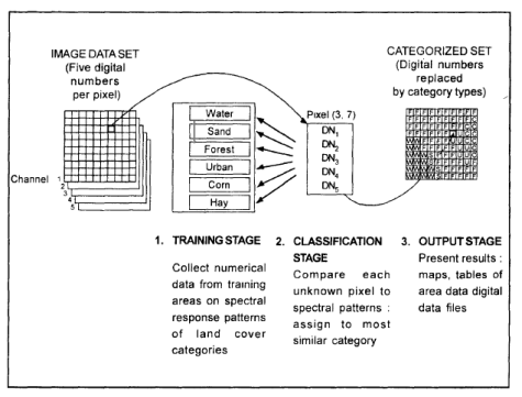
Fig. 2. Basic steps supervised classification [1]

(i) Training stage: The analyst identifies representative training areas and develops numerical descriptions of the spectral signatures of each land cover type of interest in the scene.

(ii) The classification stag(Decision Rule)e: Each pixel in the image data set IS categorized into the land cover class it most closely resembles. If the pixel is insufficiently similar to any training data set it is usually labeled ‘Unknown’.

(iii) The output stage: The results may be used in a number of different ways. Three typical forms of output products are thematic maps, tables and digital data files which become input data for GIS. The output of image classification becomes input for GIS for spatial analysis of the terrain. Fig. 2 depicts the flow of operations to be performed during image classification of remotely sensed data of an area which ultimately leads to create database as an input for GIS. Plate 6 shows the land use/ land cover color coded image, which is an output of image

2.3.1 Decision Rule in image classiffication

After the signatures are defined, the pixels of the image are sorted into classes based on the signatures by use of a classification decision rule. The decision rule is a mathematical algorithm that, using data contained in the signature, performs the actual sorting of pixels into distinct class values[2]. There are a number of powerful supervised classifiers based on the statistics, which are commonly, used for various applications. A few of them are a minimum distance to means method, average distance method, parallelepiped method, maximum likelihood method, modified maximum likelihood method, Baysian’s method, decision tree classification, and discriminant functions. Decision Rule can be classified into two types:

1- Parametric Decision Rule:

A parametric decision rule is trained by the parametric signatures. These signatures are defined by the mean vector and covariance matrix for the data file values of the pixels in the signatures. When a parametric decision rule is used, every pixel is assigned to a class since the parametric decision space is continuous[3]

2-Nonparametric Decision Rule

A nonparametric decision rule is not based on statistics; therefore, it is independent of the properties of the data. If a pixel is located within the boundary of a nonparametric signature, then this decision rule assigns the pixel to the signature’s class. Basically, a nonparametric decision rule determines whether or not the pixel is located inside of nonparametric signature boundary[3] .

2.3.2 supervised algorithm for image classiffication

The principles and working algorithms of all these supervised classifiers are derived as follow :

1. Parallelepiped Classification

Parallelepiped classification, sometimes also known as box decision rule, or level-slice procedures, are based on the ranges of values within the training data to define regions within a multidimensional data space. The spectral values of unclassified pixels are projected into data space; those that fall within the regions defined by the training data are assigned to the appropriate categories [1]. In this method a parallelepiped-like (i.e., hyper-rectangle) subspace is defined for each class. Using the training data for each class the limits of the parallelepiped subspace can be defined either by the minimum and maximum pixel values in the given class, or by a certain number of standard deviations on either side of the mean of the training data for the given class . The pixels lying inside the parallelepipeds are tagged to this class. Figure depicts this criterion in cases of two-dimensional feature space[4].

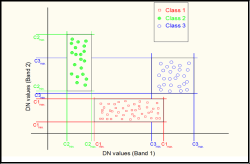
Fig. 3. Implementation of the parallelepiped classification method

for three classes using two spectral bands, after[4].

2. Minimum Distance Classification

for supervised classification, these groups are formed by values of pixels within the training fields defined by the analyst.Each cluster can be represented by its centroid, often defined as its mean value. As unassigned pixels are considered for assignment to one of the several classes, the multidimensional distance to each cluster centroid is calculated, and the pixel is then assigned to the closest cluster. Thus the classification proceeds by always using the “minimum distance” from a given pixel to a cluster centroid defined by the training data as the spectral manifestation of an informational class. Minimum distance classifiers are direct in concept and in implementation but are not widely used in remote sensing work. In its simplest form, minimum distance classification is not always accurate; there is no provision for accommodating differences in variability of classes, and some classes may overlap at their edges. It is possible to devise more sophisticated versions of the basic approach just outlined by using different distance measures and different methods of defining cluster centroids.[1]

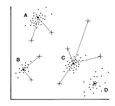
Fig. 4. Minimum distance classifier[1]

The Euclidean distance is the most common distance metric used in low dimensional data sets. It is also known as the L2 norm. The Euclidean distance is the usual manner in which distance is measured in real world. In this sense, Manhattan distance tends to be more robust to noisy data.

Euclidean distance = (1)

Where

x and y are m-dimensional vectors and denoted by x = (x1, x2, x3… xm) and y = (y1, y2, y3… ym) represent the m attribute values of two classes. [5]. While Euclidean metric is useful in low dimensions, it doesn’t work well in high dimensions and for categorical variables.

1. Mahalanobis Distance

Mahalanobis Distance is similar to Minimum Distance, except that the covariance matrix is used in the equation. Mahalanobis distance is a well-known statistical distance function. Here, a measure of variability can be incorporated into the distance metric directly. Mahalanobis distance is a distance measure between two points in the space defined by two or more correlated variables. That is to say, Mahalanobis distance takes the correlations within a data set between the variable into consideration. If there are two non-correlated variables, the Mahalanobis distance between the points of the variable in a 2D scatter plot is same as Euclidean distance. In mathematical terms, the Mahalanobis distance is equal to the Euclidean distance when the covariance matrix is the unit matrix. This is exactly the case then if the two columns of the standardized data matrix are orthogonal. The Mahalanobis distance depends on the covariance matrix of the attribute and adequately accounts for the correlations. Here, the covariance matrix is utilized to correct the effects of cross-covariance between two components of random variable[6, 7].

D=(X-M_c)^T (COV_c)^-1(X-M_c) ( 2)

where

D = Mahalanobis Distance, c = a particular class, X = measurement vector of the candidate pixel Mc = mean vector of the signature of class c, Covc = covariance matrix of the pixels in the signature of class c, Covc-1 = inverse of Covc, T = transposition function[3].

1. Maximum Likelihood Classification

In nature the classes that we classify exhibit natural variation in their spectral patterns. Further variability is added by the effects of haze, topographic shadowing, system noise, and the effects of mixed pixels. As a result, remote sensing images seldom record spectrally pure classes; more typically, they display a range of brightness’s in each band. The classification strategies considered thus far do not consider variation that may be present within spectral categories and do not address problems that arise when frequency distributions of spectral values from separate categories overlap. The maximum likelihood (ML) procedure is the most common supervised method used with remote sensing. It can be described as a statistical approach to pattern recognition where the probability of a pixel belonging to each of a predefined set of classes is calculated; hence the pixel is assigned to the class with the highest probability [4]MLC is based on the Bayesian probability formula.

Bayes’ Classification:

The MLC decision rule is based on a normalized (Gaussian) estimate of the probability density function of each class [8]. Hence, under this assumption and using the mean vector along with the covariance matrix, the distribution of a category response pattern can be completely described [9]. Given these parameters, the statistical probability of a given pixel value can be computed for being a member of a particular class. The pixel would be assigned to the class with highest probability value or be labelled “unknown” if the probability values are all below a threshold set by the user [10].

Let the spectral classes for an image be represented by

ω_i, i = 1, . . . M

Where, M is the total number of classes. In order to determine the class to which a pixel vector x belongs; the conditional probabilities of interest should be followed.

P( ωi|x), i = 1, . . . M

The measurement vector x is a column of Digital Number’s (DN) values for the pixel, where its dimension depends on the number of input bands. This vector describes the pixel as a point in multispectral space with co-ordinates defined by the DN’s (Figure 2-20).

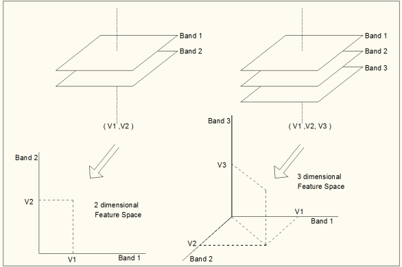
Fig. 4.Feature space and how a feature vector is plotted in the feature space [9]

The probability p(ωi |x) gives the likelihood that the correct class is ωi for a pixel at position x. Classification is performed according to:

x ∈ ωi if p ωi |x > p ωj |x) for all j ≠ i3

i.e., the pixel at x belongs to class ωi if p(ωi|x) is the largest. This general approach is called Bayes’ classification which works as an intuitive decision for the Maximum Likelihood Classifier method [11].

From this discussion one may ask how can the available p(x|ωi) can be related from the training data set, to the desired p(ωi|x) and the answer is again found in Bayes’ theorem [12].

From this discussion one may ask how can the available p(x|ωi) can be related from the training data set, to the desired p(ωi|x) and the answer is again found in Bayes’ theorem [12].

p (ωi|x)= p (x|ωi) p (ωi )/p(x) 4

Where

p(ωi ) is the probability that class ωi occurs in the image and also called a priori or prior probabilities. And p(x) is the probability of finding a pixel from any class at location x.

Maximum Likelihood decision rule is based on the probability that a pixel belongs to a particular class. The basic equation assumes that these probabilities are equal for all classes, and that the input bands have normal distributions as in [13]

D = ln(ac)-[0.5ln(|Covc|)]-[0.5(X-Mc)T(Cov-1)(X-Mc)] 6

Where:

D = weighted distance (likelihood),c = a particular class,X = measurement vector of the candidate pixel, Mc =mean vector of the sample of class c,ac =percent probability that any candidate pixel is a member ofclass c,(Defaults to 1.0, or is entered from a priori knowledge),Covc = covariance matrix of the pixels in the sample of class c,|Covc| = determinant of Covariance (matrix algebra),Covc-1 = inverse of Covariance (matrix algebra) ln = natural logarithm function = transposition function (matrix algebra).

4- Comparison supervised classification techniques:

One of the most important keys to classify land use or land cover using suitable techniques the table showed advantages and disadvantages of each techniques [3] :

5- accuracy assessment

No classification is complete until its accuracy has been assessed [10]In this context the “accuracy” means the level of agreement between labels assigned by the classifier and class allocation on the ground collected by the user as test data.

To research valid conclusions about maps accuracy from some samples of the map the sample must be selected without bias. Failure to meet these important criteria affects the validity of any further analysis performed using the data because the resulting error matrix may over- or under- estimate the true accuracy. The sampling schemes well determine the distribution of samples across the land scape which will significantly affect accuracy assessment costs [14]

When performing accuracy assessment for the whole classified image, the known reference data should be another set of data. Different from the set that is used for training the classifier .If training samples as the reference data are used then the result of the accuracy assessment only indicates how the training samples are classified, but does not indicate how the classifier performs elsewhere in scene [10]. the following are two methods commonly used to do the accuracy assessment derived from table .

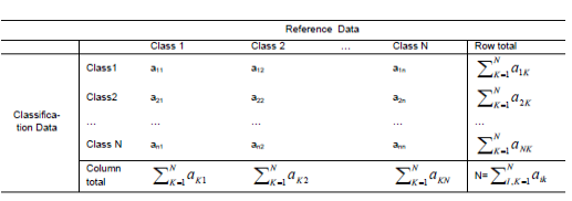1-the Error matrix

Table 1.Error matrix[15]

Error matrix (table1 ) is square ,with the same number of information classes that will be assessed as the row and column. Numbers in rows are the classification result and numbers in column are ref-erence data (ground truth ).in this square elements along the main diagonal are pixels that are correctly classified. Error matrix is very effective way to represent map accuracy in that individual accuracies of each category are plainly descried along with both the error of commission and error of omission. Error of commission is defined as including an area into acatogary when it does not belong to that category. Error of omission is defined as excluding that area from the catogary in which it truly does belong. Every error is an omission from correct category and commission to a wrong category. With error matrix error of omission and commission can be shown clearly and also several accuracy indexes such as overall accuracy, user’s accuracy and producer’s accuracy can be assessed .the following is detailed description about the three accuracy indexes and their calculation method

1. overall accuracy

Overall accuracy is the portion of all reference pixels, which are classified correctly (in the scene) that assignment of the classifications and of the reference classification agree).it is computed by dividing the total number of correctly classified pixels (the sum of the elements along the main diagonal) by the total number of reference pixels. According to the error matrix above the overall accuracy can be calculated as the following:

OA ==

Overall accuracy is Avery coarse measurement. It gives no information about what classes are classified with good accuracy.

2. producers accuracy

producer accuracy estimates the probability that a pixel, which is of class I in the reference classification is correctly classified . It is estimate with the reference pixels of class I divided by the pixels where classification and reference classification agree in class I . Given the error matrix above, the producers accuracy can be calculated using the following equation:

PA (class I) =

Producer accuracy tells how well the classification agrees with reference classification

2.3 user’s accuracy

User’s accuracy is estimated by dividing the number of pixels of the classification results for class I with number of pixels that agree with the reference data in class I.it can be calculated as :

UA(class I)=

User’s accuracy predicts the probability that a pixel classified as class I is actually belonging to class I.

2-kappa statistics

The kappa analysis is discrete multivariate techniques used in accuracy assessment for statistically determining if one error matrix is significantly different than another (bishop).the result of performing of kappa analysis is KHAT statistics (actually ,an estimate of kappa),which is an- other measure of agreement or accuracy this measure of agreement is based on the difference between the actual agreement in the error matrix(i.e the agreement between the remotely sensed classification and the reference data as indicated by major diagonal) and the chance agreement, which is indicated by the row and column totals(i.e marginal)[16]

A detailed comparison between two data sets, one with near-infrared and three visible and the other with the full 8-bands, was made to emphasize the important role of the new bands for improving the separability measurement and the final classification results [17]