Shaft Rotational Speed Experiment

Abstract:

Introduction:

Theory:

DC Generator Tachometer:

Digital Tachometer:

Stroboscope:

Lissajous Figures:

RC Filter, Low Pass:

RC Filter, High Pass:

Methodology:

Measurement System:

Sample Analysis:

Part B:

Results:

Conclusion:

Nomenclature:

References:

Appendix:

Lab Manual:

Grading Criteria:

Introduction:

 The four objectives, in their entirety, for this lab are:

• Use the least square method application (Linearity) to evaluate rotational speed.
• Random Data Analysis (Gaussian Distribution)
  • Rotation speed measurement by Digital Tachometer
• Noise Filtration: Characteristics of High and Low pass RC Filters
• Additional methods of rotational speed measurement
  • Stroboscope
  • Oscilloscope Direct Measurement
  • Lissajous Figures

Using these methods, the speed of a shaft is going to be measured. The first method is to use DC generator tachometer. Using the DC generator tachometer (electronic frequency counter), the exact speed will be able to be determined. Along with this, the voltage and frequency will be recorded. Since the relationship between the two is linear, the results of this can be used to find the rotational speed. The second method is to use a digital tachometer. To find the actual speed of the shaft using a digital tachometer requires a large data set. Then a gaussian curve of frequency distribution used to create a histogram showing where the frequencies fall. The third method is to use a stroboscope to find the shaft speed. When the frequency of the stroboscope is equal to the rotational speed of the motor, then a single line will form on the shaft face. This trend continues with two lines at double speed, three lines at triple speed. Further, this is also true if the frequency of the stroboscope is slower than the rotational speed. At half speed two lines will be observed and at a third speed, three lines will be observed.

Theory:

DC Generator Tachometer:

 By plotting the data and then using the method of least squares the relationship, $V=\mathit{ a }+\mathit{bf}$

is obtained. In this relationship $V$

is the voltage and $f$

is the frequency. The method of least squares is used to find a linear relationship between voltage and frequency. To find a and b, the following equations must be used.

$a=\frac{n\mathrm{\Sigma }{x}_i{y}_i–\mathrm{\Sigma }{x}_i{\mathrm{\Sigma }y}_i}{n\mathrm{\Sigma }{x}_i^2–{\left(x_i\right)}^2}$

$b= \frac{n\mathrm{\Sigma }{y}_i\mathrm{\Sigma }{x}_i^2–\mathrm{\Sigma }{x}_i{y}_i\mathrm{\Sigma }{x}_i}{n\mathrm{\Sigma }{x}_i^2–{\left(x_i\right)}^2}$

Digital Tachometer:

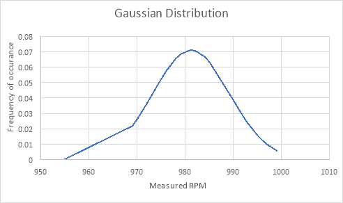
 The digital tachometer is used to obtain a large data set of the frequency. With this a gaussian curve is created. The gaussian curve shows how frequently a value occurs. It is calculated using the following equation:

$f\left(x\right)= \frac{1}{\sigma \sqrt{2\pi }}{e}^{–\frac{{(x_i–x_{\mathit{mean}})}^2}{2{\sigma }^2}}$

where,

$x_{\mathit{mean}}= \frac{\mathrm{\Sigma }{x}_i}{n}$

$\text{standard deviation},\mathit{ \sigma }=\sqrt{\frac{1}{(n+1)}\mathrm{\Sigma }{(x_i–x_{\mathit{mean}})}^2}$

Additionally a histogram of valid (within x_mean ± 3σ) data points can be plotted to show the frequency and the distribution around x_mean. The better the Gaussian curve and histogram fit, the less error there is.  To determine the amount of bins on the histogram, use Sturgis’ rule:

$\text{\# bins,}\mathit{ m}=1+3.3\log \left(N_{\mathit{valid}}\right)$

$\mathrm{size\; of\; bin},\mathrm{ \Delta }x= \frac{x_{\mathit{max}}–x_{\mathit{min}}}{m}$

 Sturges’ rule is used for determining the size of the bins. It is a very common equation used in programming for grouping data.

Stroboscope:

 The stroboscope can used to determine the speed of the rotation based on the relationship between the frequency stroboscope is flashing at and actual speed of rotation. When the frequency and the rotational speed of the shaft match, a line of light will appear on the face and appear to remain stationary. If the line is not stationary, that means either the rotational speed is slower of faster than the frequency of the stroboscope. If the line appears to be moving in the direction that the shaft is currently rotating, then the strobe frequency is faster than the speed of the rotating object. If the line appears to be rotating in the opposite direction that the object is rotating then that means the strobe frequency is slower than the speed of rotation. Below are examples of what a face might look at with vary strobe frequency vs different rotational speeds.

Stroboscope Frequency	$f$	$f$	$f$	$f$
Rotating Gear Frequency	$f$	$2f$	$\frac{1}{2}f$	$\frac{1}{3}f$
Diagram

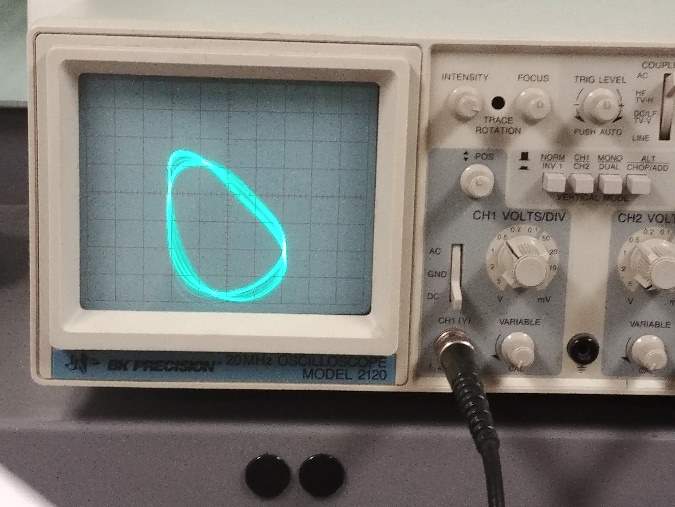
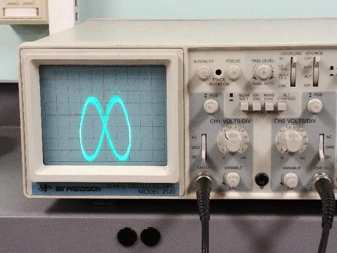
Lissajous Figures:

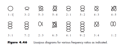
 If a known frequency is fed into an oscilloscope, then an unknown frequency also fed into the oscilloscope can be found. The known frequency, in this experiment, is on the x-axis and the unknown one is on the y-axis. By varying the unknown frequency different Lissajous figures can be observed.

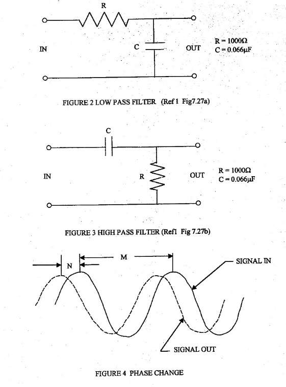
RC Filter, Low Pass:

 A low pass filter only allows frequencies below a cutoff frequency to pass through. The equation for the cutoff frequency is determined by:

$f_c=\frac{1}{2\mathit{\pi RC}}$

Output and input voltages have the following ratio:

$\frac{V_o}{V_i}=\frac{1}{\sqrt{1+{\left(\frac{f}{f_c}\right)}^2}}$

The ratio, in decibels, is equivalent to:

$\frac{V_o}{V_i}\mathit{dB}=20\log \frac{V_o}{V_i}$

Phase angle can also be determined:

$\theta =–{\tan }^{–1}\frac{f}{f_c}$

RC Filter, High Pass:

 High pass filters only allow frequencies above the cutoff to pass through. To find the cutoff frequency, voltage ratio (in decibels) and the phase angle you use the same equations as low pass filter which are, respectively, equations #, # and #. To find the voltage ratio use: $\frac{V_o}{V_i}=\frac{\frac{f}{f_c}}{\sqrt{1+{\left(\frac{f}{f_c}\right)}^2}}$

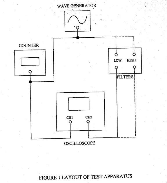
Methodology:

 There are four parts of this lab. To perform part A: “Least Square Method Application (Linearity),” one needs to do the following. First connect the magnetic pickup to the frequency counter. Second, connect the DC generator to the digital multimeter. At this time, turn on the motor and bring it to 1500 rpms. Third, turn the DC amplifier knob on the test rig to 15 volts and then lock it.  Fourth, Adjust the motor speed, in 3000rpm increments, from 1500 to 0 rpm (rotations per minute) and record the electronic frequency counter reading and the voltage on the multimeter.

 To preform part B: “Random Data Analysis: Rotating Speed by Digital Tachometer,” you must first set the motor speed to approximately 1000rpm (within 10rpm). Measure the actual speed of the shaft with the tachometer. Record both the values on the tachometer and on the digital frequency counter. A large data pool must be gathered, so repeat this step till there is enough data.

 To perform part C: “Additional Methods for Rotational Speed Measurement,” you will be measuring the speed two different ways. First by using the stroboscope, then by using Lissajous figures. For the stroboscope set the motor speed to 1000rpms. Record the electronic frequency counter reading. Set the stroboscope to the approximately the same frequency as the shaft. Record the stroboscope reading and record the gear face with either a sketch or a picture. Repeat the process for 3x and 0.5x the true shaft speed.

 To perform the second part of part C, connect the electronic frequency counter to the vertical amplifier of the oscilloscope. Set the motor speed to 1500rpm. Adjust the amplifier gain till there is a four to five-centimeter distance between the peaks of the sine waves. Without changing any settings, disconnect the input from the vertical amplifier of the oscilloscope. Connect the output of the audio-oscillator to the horizontal amplifier of the oscilloscope. Adjust the frequency of the oscilloscope to approximately the frequency of the electronic counter output. Turn the trigger control to the x-y position. Adjust either the amplitude or the gain setting of the horizontal amplifier of the oscilloscope until there is a line of approximately five-centimeters in length. Re-connect the output of the electronic frequency counter to the vertical amplifier. Sketch or photograph the resulting figure. The resulting Lissajous figure should be relatively stationary. Increase the oscillator frequency until a double loop Lissajous figure and record the frequency and motor speed which it occurs. Record the figure. Leaving the oscillator unchanged, change the motor speed until a single loop occurs. Record the figure, motor speed and oscillator frequency which this occurs.

 To perform part D: “Signal to Noise Ratio Improvement by RC Filter,” set the oscillator to 1000 Hertz. Connect the output to the electronic counter and to the input terminals A & B of the low pass RC filter. Adjust the vertical gain to produce a suitable display. After, connect the output of the low-pass filter to the channel 2 vertical input of the oscilloscope. Record the vertical peak distance and gain setting for both channels one and two, and the phase lag of the filter output with respect to the filter input signal. Repeat this process for 200; 500; 1,000; 2,000;
4,000; 8,000; 20,000; 40,000 Hertz. Then repeat the entire process with a high pass filter. Record
what lags or leads what.

Measurement System:

• D.C. Generator with Magnetic Pickup Output
• D.C. Motor
• Electronic Frequency Counter
• Digital Multimeter
• Electronic Tachometer
• Stroboscope
• Oscilloscope
• Function Generator
• Hi/Lo RC Filter

Sample Analysis:

Part A:

RPM (x)	Frequency(Hz)	Voltage(V) (y)	x2	y2	xiyi
0	0	0	0.00E+00	0.000	0
300	300	2.95	9.00E+04	8.703	885
600	600	5.9	3.60E+05	34.810	3540
900	900	8.87	8.10E+05	78.677	7983
1200	1201	11.82	1.44E+06	139.712	14184
1500	1503	14.8	2.25E+06	219.040	22200
Sums
4500	0.000	44.340	4.95E+06	480.942	48792

Using this data, apply the method of least squares.

$a=\frac{n\mathrm{\Sigma }{x}_i{y}_i–\mathrm{\Sigma }{x}_i{\mathrm{\Sigma }y}_i}{n\mathrm{\Sigma }{x}_i^2–{\left(x_i\right)}^2}$

$a=\frac{6\left(48792\right)–\left(4500\right)(44.340)}{6(4.95\mathrm{E}+06)–{\left(4500\right)}^2}=0.0099$

$b= \frac{n\mathrm{\Sigma }{y}_i\mathrm{\Sigma }{x}_i^2–\mathrm{\Sigma }{x}_i{y}_i\mathrm{\Sigma }{x}_i}{n\mathrm{\Sigma }{x}_i^2–{\left(x_i\right)}^2}$

$b= \frac{6(44.340){(4.95\mathrm{E}+06)}^2–\left(48792\right)\left(4500\right)}{6{(4.95\mathrm{E}+06)}^2–{\left(4500\right)}^2}=–0.0086$

Line of best fit:

$V=\mathit{af}+b=\left(0.0099\right)f\pm 0.0086$

Part B:

Motor Speed (Frequency Counter)	Tachometer
1004	997
998	993
999	985
997	982
996	996
996	990
993	972
996	984
991	981
989	969
992	978
992	976
991	999
992	992
991	990
991	974
989	973
991	973
993	974
993	955
989	969
989	970
988	995
982	984
995	979

Mean and standard deviation are calculated:

$x_{\mathit{mean}}= \frac{\mathrm{\Sigma }{x}_i}{n}= \frac{24530}{25}=981.2\mathit{ rpm}$

$\sigma =\sqrt{\frac{1}{(n+1)}\mathrm{\Sigma }{(x_i–x_{\mathit{mean}})}^2}=\sqrt{\frac{1}{\left(25+1\right)}\left(3133\right)}=10.977$

Data falling outside, x_mean +/- 3σ, will be rejected:

$3\sigma =32.931$

$x_{\mathit{max}}=x_{\mathit{mean}}+3\sigma =981.2+32.931=1014.131$

$x_{\mathit{min}}=x_{\mathit{mean}}–3\sigma =981.2–32.931=948.269$

 Data that resides outside of [948.269, 1014.131] can be rejected. None of the data falls outside of this range so nothing needs to be altered. Next the number of bins needs to be calculated:

$m=1+3.3\log \left(N_{\mathit{valid}}\right)=1+3.3\log \left(25\right)=5.61 \approx 6$

The Gaussian curve will be plotted using:

$f\left(x\right)= \frac{1}{\sigma \sqrt{2\pi }}{e}^{–\frac{{(x_i–x_{\mathit{mean}})}^2}{2{\sigma }^2}}=\frac{1}{(5.61)\sqrt{2\pi }}{e}^{–\frac{{(x_i–1014.131)}^2}{2(120.495)}}$

Part D:

*This is all sample data since our group didn’t have the data for this part.

Low Pass

Cutoff frequency given that R = 1000Ω and C = 0.066μF:

$f_c=\frac{1}{2\mathit{\pi RC}}=\frac{1}{2\pi \left(1000\right)(0.066*{10}^{–6})}=2,412.7\mathit{ Hz}$

The voltage ratio and phase angle are calculated:

$\frac{V_o}{V_i}=\frac{1}{\sqrt{1+{\left(\frac{f}{f_c}\right)}^2}}=\frac{1}{\sqrt{1+{\left(\frac{200}{2412.7}\right)}^2}}=0.9966$

$\frac{V_o}{V_i}\mathit{dB}=20\log \frac{V_o}{V_i}=20\log (0.9966)=–0.0296\mathit{dB}$

$\theta ={–\tan }^{–1}\frac{f}{f_c}=–{\tan }^{–1}\frac{200}{2412.7}=–4.74$

°

Using N and M phase angle can be calculated:

$\theta =\frac{N}{M}2\pi =\frac{0}{5.1}2\pi =0$

High Pass:

Cutoff frequency is the same as that of the low pass since R and C are the same. The voltage ratio and phase angle are calculated using:

$\frac{V_o}{V_i}=\frac{\frac{f}{f_c}}{\sqrt{1+{\left(\frac{f}{f_c}\right)}^2}}=\frac{\frac{200}{2412.7}}{\sqrt{1+{\left(\frac{200}{2412.7}\right)}^2}}=0.0826$

$\frac{V_o}{V_i}\mathit{dB}=20\log \frac{V_o}{V_i}=20\log (0.0826)=–21.666\mathit{dB}$

$\theta ={90°–\tan }^{–1}\frac{f}{f_c}=90°–{\tan }^{–1}\frac{200}{2412.7}=85.26$

°

Using M and N, phase angle can be calculated:

$\theta =90°–\frac{N}{M}\left(\frac{180}{\pi }\right)=90°–\frac{0.0012}{0.005}\left(\frac{180}{\pi }\right)=76.15°$

Results:

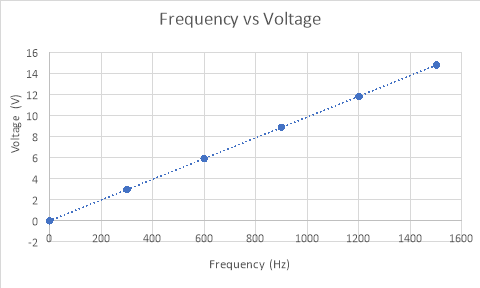
Part A:

 Using the method of least squares, a line of best fit was created to show the relationship between voltage and frequency. The graph shows that the relationship between voltage and frequency is linear. The R-squared value is 1 so the relationship is exactly, or at least within acceptable error, linear.

Part B:

Motor Speed (Frequency Counter)	Tachometer
1004	997
998	993
999	985
997	982
996	996
996	990
993	972
996	984
991	981
989	969
992	978
992	976
991	999
992	992
991	990
991	974
989	973
991	973
993	974
993	955
989	969
989	970
988	995
982	984
995	979

 

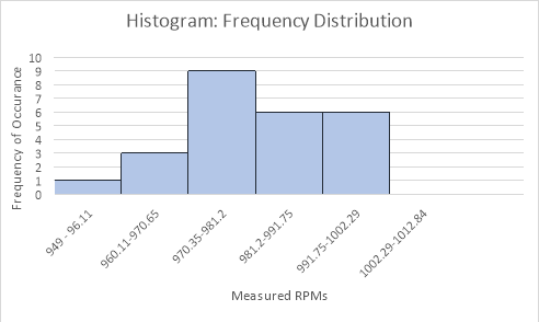
The average value found was 981.2 Hz and the actual value was 1000 Hz. This means that there is little percent error. I think the very little error we had was from pressing a little too hard with the tachometer. When it was pressed too hard, you could see the results skew.

$\%\mathit{error}=\frac{\mathit{actual}–\mathit{experimental}}{\mathit{actual}}*100\%=\frac{1000–981.2}{1000}*100\%=1.88\%$

Part C:

Stroboscope (flashes/minute)	991	1880	495	331
Rotating Gear Frequency (Hz)	990	990	990	990
Diagram

The table above shows the lines shown when the stroboscope was flashed at different frequencies at the motor. When the stroboscope’s frequency was either the same or half the rotational speed only one line showed. Two lines were visible when the stroboscope was double the rotational speed and three lines were visible when it was triple the rotational speed. 

Part D:

Conclusion:

Nomenclature:

a	Slope
b	y-intercept
C	Capacitance
f	Frequency
fc	Cutoff frequency
m	Number of bins
M	Wavelength of input voltage
N	Distance between input and output voltages
R	Resistance
V	Voltage
Vi	Input voltage
Vo	Output voltage
θ	Phase angle
σ	Standard deviation

References:

• J.p. Holman, ‘Experimental Methods for Engineers’, eighth Edition, Mc-graw Hill production, 2012, pg 60-229.
• Scott, David W. 2009. “Sturges’ rule.” WIREs Computional Statisitics. Decemeber 01. Accessed Febuary 06, 2019. http://wires.wiley.com/WileyCDA/WiresArticle/wisId-WICS35.html.
• Veen, Frederick Van. n.d. “Handbook_Stroboscopy.” IET LABS, INC. Accessed Febuary 02, 2019. https://www.ietlabs.com/pdf/application_notes/Handbook_Stroboscopy.pdf.
•  Zhu, C. (2009). ‘Rotational Speed Measurement and General Data Analysis’, ME 343 Laboratory Instructions. Newark: Mechanical Engineering Department, NJIT.

Appendix:

Lab Manual:

Safety Hazards

Instrumentation Laboratory Room 214

HAZARD:    Rotating Equipment 

                   Be aware of pinch points and possible entanglement

   Personal Protective Equipment:  Safety Goggles; Standing Shields,

   Sturdy Shoes 

   No: Loose clothing; Neck Ties/Scarves; Jewelry (remove);

          Long Hair (tie back)

HAZARD:     Projectiles / Ejected Parts

                            Articles in motion may dislodge and become airborne

       Personal Protective Equipment:  Safety Goggles; Standing Shields

HAZARD:    Heating – Burn 

                           Be aware of hot surfaces

   Personal Protective Equipment:  Safety Goggles; High Temperature Gloves; 

HAZARD:   Electrical – Burn / Shock

                           Care with electrical connections, particularly with grounding and not   using frayed electrical cords, can reduce hazard.  Use GFCI receptacles near    water.

HAZARD:    High Pressure Air-Fluid / Gas Cylinders / Vacuum

                           Inspect system integrity before operating any pressure / vacuum equipment.                            Gas cylinders must be secured at all times.  

                           Personal Protective Equipment:  Safety Goggles

HAZARD:    Water / Slip Hazard

                            Clean any spills immediately.

HAZARD:     Noise  

 

                           Personal Protective Equipment: Ear Plugs 

HAZARD:     Light Induced Epileptic Seizure

      Stroboscopic flashing light may trigger epileptic seizures in persons with                             photosensitive epilepsy

Rotation Speed Measurement and General Data Analysis

 

Objectives:

 

1. Least square method application (Linearity)
2. Random Data Analysis (Gaussian Distribution): Rotation speed measurement by Digital Tachometer
3. Noise Filtration: Characteristics of High and Low pass RC Filters  
4. Additional methods of rotational speed measurement
   1. Stroboscope
   2. Oscilloscope Direct Measurement
   3. Lissajou Figures

 

Major Equipments:  

D.C. Generator with Magnetic Pickup Output and D.C. Motor; Electronic Frequency Counter; Digital Multimeter; Electronic Tachometer; Stroboscope;

Oscilloscope; Function Generator; Hi/Lo RC Filter 

 

Procedure:  

 A. Least Square Method Application (Linearity) 

1. Connect magnetic pickup to electronic frequency counter. The counter measures rotation speed in revolution per minute (rpm), as the gear on the motor shaft has 60 teeth, which produces 60 counts per revolution.
2. Connect D.C. generator to digital voltmeter. Set motor speed to 1500 rpm on the electronic frequency counter with the motor speed control knob.
3. Turn the D.C. amplifier knob to 15.0 Volts and lock the knob on Test Rig.
4. Adjust the motor speed from 1500 to 0 rpm in interval of 300-rpm, at each point, record the electronic frequency counter reading and voltage.

 B. Random Data Analysis: Rotating Speed by Digital Tachometer

Caution: Use minimum pressure needed to record the actual shaft speed, in order to minimize the loading error and to avoid damage to the equipment.

1. Set the motor speed to 1000 ± 10 rpm (as read on the electronic frequency counter). 
2. Repeat the first step at least for 60 measurement data with each member of the team should record at least 15 readings with the digital tachometer. 

C.  Additional Methods for Rotational Speed Measurement

 

 1.  Stroboscope

 

1. Set motor speed to 1000 rpm and record the electronic frequency counter reading.
2. Set the stroboscope frequency to approximately the electronic frequency counter reading by fine-adjust the stroboscope frequency, until the timing mark appears stationary. Record the stroboscope reading, and sketch the mark on the gear face (or take a picture for record).
3. Without changing the motor speed, increase the stroboscope frequency until it is doubled. Record the stroboscope frequency. Sketch the timing mark pattern (or take a picture for record).
4. Repeat step “c” for a stroboscope frequency of 3 and ½ times true shaft speed.

 2. Lissajous Figures

1. Connect the output of the electronic frequency counter to the vertical amplifier of the oscilloscope.
2. Set the motor speed to 1500 rpm, adjust the vertical amplifier gain until a 4 or 5 cm peak-to-peak sine wave appears on the screen.  The time sweep setting can be set at any convenient value.
3. Leave the motor speed and all the setting which you just made unchanged; but temporarily disconnect the input to the vertical amplifier of the oscilloscope. Turn your attention now to the horizontal amplifier of the oscilloscope as explained below.
4. Connect the output of the audio-oscillator to the horizontal amplifier of the oscilloscope.
5. Adjust the oscillator frequency to equal approximately the frequency of the electronic frequency counter output.  Turn the trigger control to the x-y position.
6. Adjust either the amplitude setting of the oscillator or the gain setting of the horizontal amplifier of the oscilloscope, or both, until the resulting display on the oscilloscope screen will be a “line” of approximately 5 cm length.
7. Re-connect the output of the electronic frequency counter to the vertical amplifier of the oscilloscope.  The resulting Lissajous figure should remain essentially stationary, although it will be subject to some fluctuation.
8. Sketch the Lissajous figure (or take a picture for record) and record both oscillator frequency and motor speed from the electronic frequency counter.
9. Increase the oscillator frequency until a double loop figure appears (leaving the motor speed unchanged).  Sketch the Lissajous figure (or take a picture for record) and record both oscillator frequency and motor speed from the electronic frequency counter.
10. Decrease the oscillator frequency until another double loop figure appears.  Sketch the Lissajous figure and record both oscillator frequency and motor speed from the electronic frequency counter.
11. Leave the oscillator frequency unchanged and change the motor speed until a single loop appears.  Sketch the figure and record oscillator frequency and the motor speed from the electronic frequency counter.

 

D.  Signal to Noise Ratio Improvement by RC Filter

 

1. Set oscillator (frequency generator) to 1000 Hz.
2. Connect the output to the electronic counter and to the input terminals A & B of the low pass RC filter and also to CH 1 of the oscilloscope.
3. Adjust the vertical gain to produce a suitable (say 4.0 com peak-to valley) display.
4. Connect the output of the low-pass filter to CH 2 vertical input of the oscilloscope. Record:
   1. Vertical peak-to-valley CH 1 display (cm) and gain setting (volts/cm).
   2. Vertical peak-to-valley CH 2 display (cm) and gain setting (volts/cm).
   3. Phase lag of the filter output signal with respect to the filter input signal, i.e. record “M” and “N” (see Fig.4). 

Note: φ = (N)(360)/M, where φ = phase angle in degrees.

(In Fig.4, there is a phase lag φ is negative) Note: Gain Controls must be in “detent position!!

Repeat the above for the following oscillator frequency settings: (making sure that the input signal amplitude remains unchanged). 

200; 500; 1,000; 2,000; 4,000; 8,000; 20,000; 40,000 Hz

Repeat the above measurements for the high pass filter. Clearly note what lags (or leads) what. 

Grading Criteria:

MEASUREMENT OF ROTATION AND DATA ANALYSIS

Grading Criteria for Lab Report 1

(Maximum possible: 50 points + Bonus: 15 points)

1.  General Format: (15 points = 2.5+5.0+2.5+5.0)

• Cover page (2.5 points)
• Grading Criteria
• Abstract
• Introduction
• Table of contents (Include “Responses for Bonus points”, if any, after Conclusion) Table of Figures
  • Schematic diagram of experimental system
  • Actual images (photographs) of the system, key components, & results as applicable
• Results and Discussions (See details & scores shown below separately)  Conclusions (2.5 points)
• Appendices (5.0 points)
  • Lab manual
  • Photocopy of original data (as applicable)
  • Detailed sample calculation
  • Nomenclature used in report
• Use PAPER folder with brads (no plastic or three ring binder or staple(s))

2. Results and Discussions: (35 points = 10+15+10)

• DC Voltage versus rotation speed (10 points = 5.0+2.5+2.5)
  • Plot of data (DC voltage vs. speed) (5.0 points)
  • Least square method (2.5 points)
  • Data-fitted equation (with uncertainty) from least-square method (2.5 points)

• Random data analysis using measurements of digital tachometer: (15 points = 6×2.5)

Collect 25 measurements per student using tachometer – tabulate

• Mean & standard deviation – use excel Data Analysis (2.5 points)
• Mean and standard deviation using Excel spreadsheet + typed formulas (2.5 points) Use Minitab & get Histogram with normal distribution curve (2.5 points)
• In generating the Histogram use Sturges’ rule & discuss Sturges’ rule (2.5 points) Compare PDF against Gaussian distribution (68%, 95%, 99.73%) (2.5 points)
• Data validation (2 rule) exclude any bad data (use only 2 data) (2.5 points)

 

• Other speed measurements: (10 points = 2.5+5+2.5):
  • Stroboscope: estimate the average speed Include expected sketch / observed photograph, discuss (2.5 points)
  • Direct oscilloscope measurements: graphical determination – determine the equation for the waveform displayed (one speed per student) (5 points)
  • Lissajous figures: graphical comparison – expected sketch / observed Photograph, discuss (2.5 points)

 

 3. Bonus Questions:  (15 points = 2.5+2.5+5+5):

• When you use the stroboscope what makes the image of the white line seem to drift slowly rather than remain stationary? (answer should include sketches & should not exceed one page) (2.5 points)
• What do you understand by the term ‘Kurtosis’ – discuss its meaning & significance (answer should include sketches of normal distribution curves, and should not exceed one page) (2.5 points)
• What is more important: Mean or Standard deviation in analyzing a set of data (answer should include sketches of normal distribution curves, and should be about one page) (5 points)
• What do you understand by the term ‘six sigma’ (answer should include sketches of normal distribution curves, and should be about one page) (5 points)