Reynolds Averaged Navier Stokes (RANS)
| ✅ Paper Type: Free Essay | ✅ Subject: Engineering |
| ✅ Wordcount: 2917 words | ✅ Published: 30 Aug 2017 |
Before Computational Fluid Dynamics(CFD) was developed, theoretical studies on high swirling confined turbulent flows can only be validated by conducting experimental studies. These experimental studies require long leading time and high cost. Now, with the help of CFD, researchers are able to study these complex flows in a much shorter time and with a lower cost incurred.
Many experimental studies have been conducted on the high swirling confined turbulent flows but little has been done on the computational modelling. Most of these intricate flow simulations are accomplished at the expense of high computational cost methods such as Large Eddy Simulations(LES) and Direct Numerical Simulations(DNS). Thus, a lower computational cost alternative will be very helpful in the studies of high swirling confined turbulent flows.
Thus, this project will be using the Reynolds Averaged Navier Stokes (RANS) based turbulence models in ANSYS FLUENT to simulate the high swirling confined turbulent flows in two different test cases and the results validated with experimental data. The aims and objectives are discussed as follows:
Aims and Objectives
Aims
To validate the accuracy of RANS based turbulence models for the simulation of high swirling confined turbulent flows.
Objectives
- To simulate the high swirling confined turbulent flows using ANSYS FLUENT with different RANS turbulence models.
- To compare the numerical data from the simulations with the experimental data to validate the accuracy of the turbulence models.
- To understand the effect of the RANS turbulence models on the predicted results.
Review of Confined Swirling Flows
Confined swirling flow plays an important role in various engineering fields. For example, they can enhance the mixing process in the stirred tanks, improve the separation of particles in cyclones [1] and also increases the flame stability in gas turbine combustors. So, what is a swirling flow?
A swirling flow is a flow where a swirl velocity that exists in the tangential direction other than the flow motion in the axial and radial directions. The swirl velocity of the flow plays a major role in the evolution and decay process of swirling flow motion but not the radial velocity of the flow as shown in a study by Beaubert et al. [2]
A swirling flow consist of two types of rotational motion. A solid body rotation at the inner region near the centerline and a free vortex motion at the outer region. [14] Solid body rotation and free vortex motion respectively has its velocity directly and inversely proportional to the radius of the pipe at the centre of their axis of rotation as shown in Figure 1.
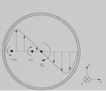
Figure 1: Velocity profile of swirling flow in a pipe. [4]
Confined swirling flow can then be categorized into “subcritical” and “supercritical” flows. A “subcritical” flow has a reverse flow at the exit and is very sensitive towards changes at the exit as shown experimentally by Escudier and Keller[11]. On the other hand, the “supercritical” flow has no reverse flow at the exit and is insensitive towards variation at the exit.[10] “Subcritical” flows are formed when the ratio of maximum swirl velocity to the averaged axial velocity exceeds unity was stated in a theory by Squire[12].
Review of Computational Fluid Dynamics(CFD)
CFD is a methodology which is employed to study fluid flow using numerical analysis and algorithms to solve the governing flow equations. In the past, the field of fluid dynamics was made up of purely experimental and theoretical studies. CFD is considered the “third approach” in the studies of fluid mechanics and would complement the two existing methods. [5]
The three main elements when implementing CFD are the pre-processor, solver and post-processor. The pre-processor’s task is to transform the input of a flow problem into a form that is suitable for the solver. During pre-processing, the geometry of the problem is defined and the flow domain is divided into smaller cells (meshing). The physical (eg: turbulence) and chemical phenomena that needs to be modelled are selected and the fluid properties are defined. Next, the boundary conditions are given to cells which interacts with the domain boundary. The solution to the flow problem is stored in the nodes in each cell. In the solver, the conservation equation containing the mass, momentum, energy and species is integrated over each cells. Then, the unknown variables of the equation are interpolated and substituted back into the equation. The solver then runs numerical techniques to solve the derivatives and flux in the cells. Lastly, the post-processor allows user to analyse the data obtained by plotting graphs and observe the flow animation. [6]
Review of Turbulence Flows
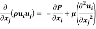
All fluids in motion are governed by the conservation of mass equation and the Navier-Stokes equation. The latter equation relates the flow properties such as the velocity, pressure, density and temperature for a moving fluid. The conservation of mass equation and the incompressible Navier-Stokes equation (in Cartesian tensor notation) can be respectively written as

Turbulence is shown to develop as an instability in the laminar flow through detailed analysis of the solutions for the Navier Stokes equation. [7].
In principle, Direct Numerical Simulation(DNS) can be used to simulate very accurate turbulent flow by solving the exact equations with the appropriate boundary conditions. However, it requires very large amount of computational power as this method has to represent all of the eddies from the smallest scale to the largest scale and the time step chosen must be small enough to resolve the fastest fluctuations. The turbulent eddies will be discussed in more detail in the next section.
The two other methods that can be used to simulate the turbulent flows (with decreasing computational power and accuracy) would be the Large Eddy Simulation(LES) and turbulence modelling with Reynold’s Averaged Navier Stokes equation (RANS). Basically, LES solves the governing equations partially as only the large eddies are solved using the governing equations and the filtered smaller eddies are modeled while RANS models the entire turbulence eddies and only the mean variables are calculated.
For turbulence modelling, the minute details of the turbulent motion are not prioritized so only the average flow properties are solved. In a turbulent flow, the velocity field fluctuates randomly in both space and time. Despite the fluctuations, the time averaged velocity can be determined and the velocity field equation can be written as:
 (
( )
)
where  is the time averaged velocity and
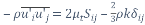
  is the fluctuating component in the velocity field. Other than the velocity, other flow properties can also be decomposed into its mean and fluctuating parts. In our simulations, the flow is assumed to be steady, have constant density and axially symmetric. Thus, the incompressible Reynold’s Averaged Navier-Stokes (RANS) equations (in Cartesian tensor notation) can be written as

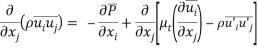
Where  is the Reynold’s Stress tensor,
 which is a component of a symmetric second order tensor from the averaged process. The diagonal terms are normal stresses while the non-diagonal terms are shear stresses. The Reynolds Stress can be understood as the net momentum transfer due to velocity fluctuations. This term also provided unknown terms to be equation and thus, more equations have to be found to match the number of unknowns to solve the equations.
A straightforward method of “generating” equations would be to create new sets of partial differential equations (PDEs) for each term using the original set of Navier-Stokes equation. This can be done by multiplying the incompressible NS equations by the fluctuating property and time averaging them to produce the Reynolds-Stress equation. By deriving the Reynolds Stress term, we can identify what is influencing the stress term but the problem with this approach is that more unknowns and correlations were generated and no new equations are formed to account for these unknowns. [7] Thus, these unknown terms have to be modelled to close the equation before they can be used.
Review of Turbulence Eddies
The velocity field fluctuations in the turbulence flows are actually the eddies in the flow. The eddies moving pass an object generates the turbulence kinetic energy and the length scale of the eddies, are determined by the diameter of the object. As the large eddy break down into smaller eddies, the turbulence kinetic energy will be passed down and eventually dissipated due to viscous forces in the flow. Thus, according to the Kolmogrov scales, the length and time scale of the smallest eddies depends on the rate they receive energy from the larger eddies,
  and the kinematic viscosity,
 . It is also noted that the rate of turbulence energy received is equal to the rate of turbulence energy dissipated so,
  . The Kolmogrov scales shows the length and time scale of the smallest eddies to be
  and
and  respectively. [8] These expressions can then be used to determine the length and time scale ratio between the small and large eddies.
 (
( )
)
 (
( )
)
From the equations above, we can conclude that the large eddies are several orders of magnitude larger than the small eddies. Thus, even at a low Reynold’s number, the time and length ratio between the small and large eddies are significant enough to affect the number of elements and time step required to model the entire turbulent flow. Therefore, instead of solving all the eddies, turbulence modelling is required to reduce the amount of computational cost of CFD.
Summary
The understanding of the motions of confined swirling flows and characteristic of the “subcritical” and “supercritical” flows will be useful when explaining the simulation results. Before the simulation results are obtained, it is also important to identify the basic steps of running any CFD simulations which are the preprocessing, solving and post processing.
DNS solves the exact NS equation while LES solves the equation for larger eddies and models the smaller eddies. The process of solving the exact equations takes up a lot of computational power as it would need to represent the all the turbulent eddies involved and a suitable time step has to be chosen to resolve the fluctuations. When compared to DNS and LES, RANS turbulence modelling requires the least computational power as it does not solve the exact NS equations but instead, models the entire turbulence eddy and only solves the mean average variables. The low computational cost of RANS turbulence modeling is the primary reason why this project has chosen it to simulate the confined swirling flows. However, the accuracy of this methods requires validation, which is the aim of this project.
The RANS turbulence models created will be based on the PDEs of the Reynolds stress as a guideline as it shows how the Reynold stress behave. Thus, the next section will elaborate more about the RANS turbulence models that will be implemented in this project.
The main objective of the RAN based turbulence models are to model the  (Reynold’s Stress tensor) and provide closure to the RANS equation. The three main categories of the turbulence models are linear eddy viscosity models, non-linear viscosity models and Reynolds’ Stress Model(RSM). [9]
There are three types of linear eddy viscosity models: algebraic models, one equation models and two equation models. They are based on the Boussinesq hypothesis which models the Reynold’s stress tensor to be proportional to the mean rate of strain tensor, by a coefficient named the eddy viscosity,
 . This infers that the turbulence flow field acts similarly to a laminar flow field. [10]
 (5)
(5)
The second term of the right hand side of the equation above is required when solving turbulence models that needs to calculate the turbulent kinetic energy, k from the transport equations. The equation for k is half the trace of the Reynolds Stress tensor.

For the algebraic turbulence models, no additional PDE equations are created to describe the transport of the turbulent flux and the solutions are calculated directly from the flow variables. An algebraic relation is used as closure based on the mixing length theory. The mixing length theory states that the eddy viscosity have to vary with the distance from the wall. However, the problem with these equations are that they do not account for the effects of turbulence history. In order to improve the turbulent flow predictions, an additional transport equation for k is solved which will replace the velocity scale and include the effects of turbulence flow history.
For one and two-equation models, the modeled k equation is involved thus discussion on the exact k equation will first be done. The exact k equation is a PDE derived by multiplying the incompressible NS equations with  , averaging it and multiply with
  . The exact k PDE equation obtained is
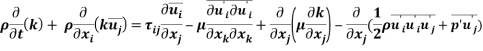
The left hand side(LHS) terms are the material derivative of k which gives the rate of change of turbulent kinetic energy. The first term on the right hand side(RHS) is the production term and represents the turbulent kinetic energy that an eddy will gain due to the mean flow strain rate. The second term on the RHS represents the dissipation term which meant the rate at which the kinetic energy of the smallest turbulent eddy being transferred into thermal energy due to the work done by the fluctuating strain rate against the fluctuating viscous stresses. The third term on the RHS is the diffusion term which represents the diffusion of turbulent energy by molecular motion. The last term of the RHS is the pressure-strain term which signifies the tendency to redistribute the kinetic energy in the flow due to the turbulent and pressure fluctuations. In order to close and solve the k equation, the Reynolds Stress, dissipation, diffusion and pressure-strain term has to be specified.
For the Reynolds Stress term, it is already mentioned at the beginning that it is based on the Boussinesq hypothesis. The eddy viscosity, is modelled similarly to how it was done for the algebraic models

Where  is a constant, the length scale of turbulence eddies,
  is similar the mixing length and velocity scale of the turbulence eddies is replaced by the square root of the turbulence kinetic energy, k. The equation above is an isotropic relation which means that it is assumed that the momentum transport is the same in all direction at any point.
Next, the dissipation term is modelled based on the assumption that the rate of turbulence energy received is equal to the rate of turbulence energy dissipated. Thus, we can write the equation
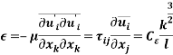
and since the equation is homogenous, it can be characterized by the length and velocity scale of turbulence eddies giving

Where  is a constant.
For the diffusion and pressure-strain term, the sum is modelled based on the gradient diffusion transport mechanism as there is the pressure-strain term is small for incompressible flows. The gradient transport mechanism implies that there is a flux of k down the gradient. It is to help ensure that the solutions are smooth and a boundary condition can be applied on k when k is in the boundary. There is no Therefore, the equation shows
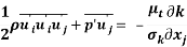
Where  is the turbulent Prandtl number and is normally equal to one.
-not completed
– will talk about the modeled turbulent kinetic energy in one equation spalart allmaras
-will talk about dissipation part for 2 equation model in k-e
This test case is chosen because the flow was mapped and documented in detail as So et al was able to measure and document the flow in detail using a Laser Doppler Velocimetry(LDV) at 10 axial stations up to 40d downstream. Thus, the validation of the accuracy of the RANS turbulence models on confined high swirling flow can be done.
Description of Test Case
The flow consists of an annular high swirling stream projected into a pipe of uniform radius, R = 62.5mm with a central non-swirling jet of diameter, d = 8.7mm. The swirl number, S of the flow is calculated with
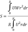
Where U is the axial velocity and W is the swirl velocity. The swirl number just downstream of the swirl generator is approximately 2.25 which indicates that it is a high swirling flow and will cause an adverse pressure gradient at the centreline. The purpose of the non-swirling jet was to delay the occurrence of reverse flow due to the adverse pressure gradient along the centreline from 12d to 40d downstream from the inlet.
Geometry (Computational Domain)
The confined swirling flow in this case is a “subcitical” flow according to the rule of thumb of Squire mentioned in Section x. Thus, two different computational domains were used for the simulation of the flow to check if the exit geometry will affect the swirling flow simulated.
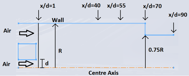
Figure 2 (temporary figure)
The first computational domain is the complete geometry of the pipe which consist of the computational inlet at x/d =1 and the constriction of 0.75R from x/d = 70 to the computational outlet at x/d = 90. The second computational domain is a “cut” off from the first domain at x/d = 55 where the constriction is removed.
Meshing
-have not completed it. Will be updated in the next revision.
Boundary Conditions
Inlet
The inlet experimental measurements for the axial and tangential velocity and stresses are provided. However, the radial velocity component was not measured and is set to 0 rad/s. The radial stress is also not measured and was set equal to the tangential stress, whereas the three shear stresses are assumed to be zero. < graphs of prescribed to be added>
Outlet
Conditions at the outlet are not known prior to solving the flow problem. No conditions are defined at the outflow boundaries as ANSYS FLUENT will extrapolate the required information from the interior. It is assumed that the flow is fully developed at the exit end thus the outflow boundary condition is used. (dphi/dx|exit = 0)
Wall
The no slip condition is applied.
Cite This Work
To export a reference to this article please select a referencing stye below:
Related Services
View all


DMCA / Removal Request
If you are the original writer of this essay and no longer wish to have your work published on UKEssays.com then please click the following link to email our support team:
Request essay removal