Multi-objective Optimization Mathematical Model

CHAPTER 3 PRODUCTION COST & WORK INJURY LEVEL MODELLING

3.1 Introduction

This chapter describes a multi-objective optimization mathematical model with decision variables and constraints on them. Section 3.2 presents the model formulation with aim to minimize the total production cost and work injury level particularly in a manufacturing industry over a planning horizon. Section 3.3 presents [ZC1]the case study drawn from literature to validate the proposed model. Section 3.4 presents the method to calculate the work injury cost with consideration of work injury level factor. Section 3.5 gives the summary for this chapter.

Model formulation

The traditional production planning model is a mathematical optimization model. In such a model, the objective function is the total cost, and the decision variable refers to production quantity, inventory quantity, and outsourcing quantity. The constraint function in the traditional production planning model includes the demand in a planning horizon. In the work of (Xu, 2015), the traditional model includes the work injury cost. The expansion of the model hence mentions the description of the objective function and constraints. The model aims to achieve the two objective are:

• Objective 1 (ob1): Minimize production cost (C_P).
• Objective 2 (ob2): Minimize work injury level (WIL).

Model Assumptions

A mathematical model herein is developed on the following assumptions are:

1. The values of all parameters are certain over the next period t in planning horizon.
2. Actual labor levels, working hours and warehouse capacity in each period cannot exceed their respective maximum levels.
3. The number of workers and tasks are the same over the planning horizon.
4. A single type of product is manufactured over the planning horizon.
5. Trivial solutions will be ignored.

Model Notations

The following notations are used after reviewing the literature and considering practical scenarios (Wang & Liang, 2004; Masud & Hwang, 1980; Wang & Fang, 2001; Chakrabortty & Hasin, 2013).

t: the time period (t=1, 2, 3, …, n).

C_MR: the regular unit material cost of the product ($/unit).

C_MO: the overtime unit material cost of the product ($/unit).

P_t: the number of products fabricated (production quantity) during the regular working hours in the period t (unit).

O_t: the number of products fabricated (overtime production quantity) during the overtime in period t (unit).

C_LR: the regular unit labor cost in period t ($/unit).

C_LO: the overtime unit labor cost in period t ($/unit).

H_t: the regular working man-hour required in period t (man-hour).

E_t: the overtime working man-hour required in period t (man-hour).

C_I: the unit inventory cost ($/unit).

I_t: the units of product to be left over as an inventory during period t (unit).

C_WI: total work injury cost over the planning horizon.[C2]

[aa3] I_t-1: the units of leftover products in the previous period of t.

d_t: the product demand in period ‘t.’

D: the total demand over the planning horizon.

d_n: the number of working days in period t.

W :the number of employees.

E* : allowable overtime hours in period t.

Objective function (ob1)

To achieve the ob1, the integrated production planning was used in order to minimize the production cost. The total production cost consists of the material cost, labor cost, inventory cost and work injury cost. Let C represent various costs. The total cost is hence denoted by:

(3.1)

[ZC4]

where

C_production: the total production cost.

C_material: the material cost.

C_labor: the labor cost.

C_inventory: the inventory cost.

C_WI: work injury cost.

where

• Material Cost: Material cost is the sum of regular material cost and overtime material cost that includes the raw material cost and overhead cost. Raw material directly contributes to the finished product, and the overhead cost includes the utility cost such as electricity, gas and rent etc.

• Labor Cost: Labor cost is the sum of all wages paid to employees for the production of products in both regular time and overtime hours.

• Inventory cost: Inventory cost is the holding cost of products in stock.

• Work injury cost: the work injury cost caused by the repetitive assembly production over an entire production period

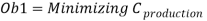
The first objective function (ob1) of the model is to minimize the cost of production (eq. 3.2).

(3.2)

(3.3)

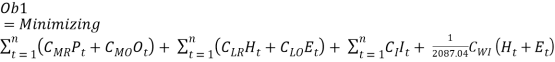
Moreover, equation 3.1 can be written as:

[ZC5][aa6]

Where, the first part of equation 3.3, 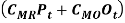represents the regular material cost (C_MR) incurred on the regular production quantity (P_t) and overtime material cost (C_MO) on overtime production quantity (O_t) over the planning period. The second part 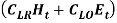represents the labour cost (worker’s salary) and it is the combination of the regular unit labor cost (C_LR) during regular working hours (H_t) and the overtime unit labor cost (C_LO) in overtime working hours (E_t). The third part is the unit inventory cost for left over products as an inventory over the period (I_t) and the final part denotes the accumulated work injury cost (C_WI) during regular working man-hour (H_t) and the overtime working man-hour (E_t). Furthermore, the C_wiis calculated on a yearly basis with 21.74 working days in a month and 8-hour shift as per the study by Lin. (2008). It can be seen in equation ().

(2)

Objective function (ob2)

The second objective function (ob2) of the modelis to minimize the work injury levels over the planning horizon as shown below;

Furthermore

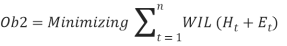
Where, equation () represents the accumulated work injury level (WIL) during regular working man-hour (H_t) and the overtime working man-hour (E_t) in the time period t. As discussed in literature that increase in regular and overtime production quantity will increase the work injury level because of long exposure of worker to the repetitive task. Therefore, higher the production quantity, the longer the working hours and the higher the work injury level.

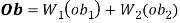
Overall objective function

Decision variables

The decision variables in the above model are explained below:

• Production quantity (P_t) during the regular working time in period t.
• Overtime production quantity (O_t) in period t.
• Number of products in inventory (I_t) in period t.

Dependant variables

• Regular working man-hour (H_t) required in period t.
• Overtime working man-hour (E_t) required in period t.

3.2.3 Constraints

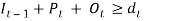
• Demand constraint

(3.4)

(3.4)

Where, the sum of regular production quantity (P_t), overtime production quantity (O_t) and inventory levels essentially greater than or equal to the market demand (d_t) in a period ‘t’ as shown in equation 3.4. Moreover, the sum of all periods demand (d_t) should be greater than or equal to total demand (D) over planning horizon as shown in equation 3.4.

• Labor hour limit constraint.

(3.5)

where, equation (3.5) represents the regular working man-hour (H_t) in period ‘t’ should be less than or equal to 8 hours per day, monthly working days (d_n) as well as number of employees (W). Overtime working man-hour (E_t) should not exceed the allowable hours (E*) by law.

• Production rate constraint. Assume that the unit time is one hour, and the relation between the produced units and labor can be expressed as:

(3.6)[C7]

where

R_h: the production rate during regular working time.

R_e: the production rate during overtime.

• Non-negative constraints. The number of produced product, the number of demand and the unit labor cost are non-negative, respectively that is:

(3.7)

Model implementation

To validate the model efficiency, the specific case study about the aggregate production planning of single product is selected. This case study is drawn from the literature and the author’ s own experience in industry (Chakrabortty & Hasin, 2013).

Case study description

To validate the proposed model, the real life data of Comfit Composite Knit Limited (CCKL) is taken. The company manufactures knit ware product. The production planning is more specifically about the production of ‘hooded jacket’ over a couple of months planning horizon. Table 3.1 & 3.2 give the monthly product demand, and related cost data are as follows.

Table 3.1 Product demand over planning horizon

Period (t)	May	June
Demand (dt) (units)	1400	3000

Table 3.2 Cost data of case study

Regular time unit material cost (CMR)	14 ($/unit)
Overtime unit material cost (CMO)	28 ($/unit)
Inventory Cost (CI)	3.5 ($/unit)
Regular time unit labor cost (CLR)	8 ($/unit)
Overtime unit labor cost (CLO)	12 ($/unit)

.

Table 3.3 Model Constraint Data:

Initial Inventory level- I0	500
End inventory in period- I2	400
Labor hour (Ht 0+ Et)	≤ 225 man-hours
Production rate (Rh)	0.033 man-hour/unit

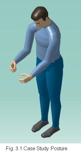
In given case study, the company makes knit ware product (Hooded Jacket). In manufacturing of product, the job requires a worker posture in a standing position to process the product on a machine. The worker need to place the product parts in a machine to stitch it , for this reason worker has to lean forward to focus on the product parts. The neck may bend to get a better view of stitching if required. To perform this task, the upper arms are need to be elevated to the height of the work table. To place the product part in a right way the body rotation is required (Fig. 3.1).

3.3 Work injury cost (C_wi) calculation

Work injury cost [C8](C_wi) is calculated by using the model proposed by Lin (2008). This model is shown here (Eq. 3.8):

(3.8)

where

C_WI: the cost of work injuries;

α_n: the coefficient of multiplier associated with each variable X1 to X_7.

X1: the type of business Manufacturing; M61; 1: Mills and Semi-medium

0: otherwise;

X2: the type of business M81; 1: Metal Foundries and Mills; 0: otherwise;

X3: the type of business M91; 1: Agricultural Equipment; 0: otherwise;

X4: the type of business M92; 1: if it is Machine Shops, Manufacturing;

0: otherwise;

X5: worker’s age.

X6: gender; 1: if it is male; 0: otherwise;

X7: the level of work injury.

ε: the error term.

The work injury levels of different body parts are presented in Table 3.13 (Lin, 2008).

Table 3.13 Work injury level range

Parts of Body	Level of work injury
Upper Arm	1-6
Forearm	1-3
Wrist	1-4
Neck	1-6
Trunk	1-6
Leg	1-7

The statistics software SPSS® is used (Lin, 2008) to determine the coefficient of every variable in equation 3.8. In the first step, all data regarding each variable were redefined. In the second step, work injury cost (dependent variable) was adjusted by power transformation. Hence, the work injury cost model is expressed by the following equations (Lin, 2008).

		(3.9)
	(3.10)
	(3.11)
	(3.12)
	(3.13)
	(3.14)

After the second step, Equation 3.9 to 3.14 were again adjusted to calculate the work injury cost. The manufacturing type of business is considered, therefore X1=X2=X3=0 and X4=1. It has been noticed that the age and gender coefficient were small and can be neglected. Furthermore, the equation states that work injury levels were the major part in work injury cost (Xu, 2015). The revised work injury cost model equations are as follows;

	(3.15)
	(3.16)
	(3.17)
	(3.18)
	(3.19)
	(3.20)

From the above discussion, it was noticed that to calculate the work injury cost the first step is to measure the work injury level of a given posture. Moreover, in order to measure the work injury level (WIL), DELMIA®V5 production software (Lin,2008) is used. In the first step, “Human Builder” tool is used for posture visualization. In the second step, posture simulation is done by using “Posture Editor” tool. In the last step, to measure work injury level for the particular posture “RULA” (Hedge, 2001) is applied.

3.5 SUMMARY

In this chapter, multi objective optimization model was tailored to achieve desired objectives. First objective was to minimize the total production cost over the planning horizon with consideration of work injury cost factor. Second objective was to minimize the work injury levels over the planning horizon. In Section 3.2 multi objective optimization was made along with decision variables and constraints on them. Assumptions and notations were taken from Chakrabortty & Hasin. (2013), Wang et al. (2005) and Xu. (2015). In the next Section 3.3 the case study was presented to validate the model. In Section 3.4 work injury cost calculation method was presented with its all variables and work injury level range. Thus, both objectives 1 & 2 mentioned in chapter 1 have been achieved by proposed model. More detail regarding the results will be discussed in next chapter.