Levelized Cost of Energy (LCOE) Model for Wind Farms
| ✅ Paper Type: Free Essay | ✅ Subject: Engineering |
| ✅ Wordcount: 4683 words | ✅ Published: 31 Aug 2017 |
A Levelized Cost of Energy (LCOE) Model for Wind Farms with Power Purchase Agreements (PPAs)
The cost of energy is an important issue in the world as demand for renewable energy resources is growing. Performance-based energy contracts are designed to keep the price of energy as low as possible while controlling the risk for both the Buyer and the Seller. Price and risk are often balanced using Power Purchase Agreements (PPAs). Since wind is not a constant supply source, in order to keep risk low, wind PPAs contain clauses that require the purchase and sale of the energy to fall within reasonable limits. However, the existence of those limits creates pressure on prices, causing increases in the Levelized Cost of Energy (LCOE). Depending on the variation in capacity factor (CF), the power generator (the Seller) may find that the limitations on power purchases required by the utility (the Buyer) are not favorable and will result in higher costs of energy than predicted. Existing LCOE models do not take into account energy purchase limitations or variations in energy production when calculating an LCOE. The challenge addressed in this paper is that the price schedule in a PPA is determined using the LCOE provided by the Seller, but the energy delivery limits imposed within the PPA impact the LCOE in ways that are not accommodated by existing models.
A new cost model has been developed to evaluate the price of electricity from wind energy under a PPA contract. This paper presents a method that an energy Seller can use to develop an appropriate Cost of Energy (COE) based on desired energy delivery quantities. The new cost model can then be used as a basis for setting an appropriate PPA price schedule. During the PPA negotiations, LCOE is calculated and used by the seller to determine an appropriate COE for each unit of energy that falls within the conditions set within the contract. As the COE isnegotiated and determined to be too high or too low by either party, the PPA terms are changed to adjust for the desired PPA prices. PPA energy purchase limitations can change the LCOE by as much as a factor of two depending on the energy limitations. The application of the model on real wind farms shows that the actual LCOE depends on the limitations on energy purchase within a PPA contract as well as the expected performance characteristics associated with wind farms.
Cost of Energy (COE) becomes a major concern for the public and utilities as the demand for power from renewable energy sources, such as wind, increases. Utilities may become reluctant to purchase more renewable energy than they are required to purchase if the COE is too high. COE is the actual cost to buy energy while LCOE is the break-even cost to generate the energy. The LCOE is a commonly accepted calculation of the Total Life-Cycle Cost (TLCC) for each unit of energy produced in the lifetime of a project[1].
In addition to the increase in the use of renewable energy sources, there is an increase in the use of PPAs for all sources of energy. PPAs are Performance-Based Contracts (PBCs) that aim to create a “fair” agreement for the purchase and sale of energy between a utility (the Buyer) and a generator (the Seller). The use of PPAs has been increasing around the world and they are commonly used in Europe, the U.S., and in Latin America. In Germany alone, offshore wind projects with PPAs totaled over 1.2 GW in capacity in 2013[2]. In the U.S. there existed a total of 29,632 MW of capacity in 343 signed or planned PPAs in 2014-2015[3]. Between 2008 and 2016, 650 MW of new capacity was signed in the U.S. and in 2015 the use of PPAs in the U.S. grew to 1.6 GW[4]. In Latin America, the government typically awards PPAs. In 2014, the government of Peru awarded PPAs to projects with a total of 232 MW of capacity[5]. `
PPAs use an LCOE calculation to determine a fair price of energy, much like a standard retail energy contract[1]. However, Buyers in a PPA can create terms that limit the annual purchase of energy, thereby affecting the actual LCOE. Buyers can create a limit for the minimum annual amount of energy that needs to be delivered and/or the maximum amount that energy will be bought at full price. The PPA contract limits create penalties; a penalty is incurred when the Seller does not fall within the energy delivery requirements. In a normal energy contract (such as a standard retail contract, a market retail contract, and in a PPA), the LCOE is calculated over the period of the contract and energy is purchased as it arrives at the agreed upon point of delivery. PPAs are used to share and reduce the risks of added costs, however, in some cases the costs are not accounted for within LCOE models.
Conventional LCOE models include all the costs associated with an energy project. PPAs address and outline the capital costs, operational costs over the lifetime of the project, the energy produced, tax credits, and the weighted average cost of capital (WACC) within a specific project.[2] The National Renewable Energy Laboratory (NREL) and others have developed and used LCOE models that typically consider all or most of these parameters [6][7][8]. The terms of the PPA are important because they create costs that affect the actual LCOE. However, current LCOE models do not include the effects of the energy delivery limits and their penalty costs imposed by PPAs as a cost to the wind farms. If the LCOE does not reflect the break-even cost, the Seller risks the project’s failure and the Buyer risks the loss in profit from not providing enough energy to its end-use consumers. A more accurate LCOE could prevent the failure of a wind farm and benefit the Seller, the Buyer, and consumers.
In this paper, a new LCOE model is proposed to address the PPA annual energy delivery limits, which we refer to as penalties. Although the application of penalties as a cost appears to be straightforward (because of their direct and indirect costs to the Seller), the penalties are more complex to analyze when uncertainties are introduced. The difference between the LCOE with and without penalties can be significant (see the Wind Farm Case Study). The effect of penalties on the LCOE can vary depending on the capacity factor (CF), the variation in CF, as well as the limits on the purchase of energy. Determining the best limits in a PPA depends on the needs of the Buyer in conjunction with a desire for a COE that reflects the actual LCOE for the Seller within the contract. This paper develops a method that provides a tool that the Seller can use to negotiate penalties and an appropriate COE within their PPAs.
PPAs define every aspect of the project including: the terms for the entire project’s construction, operation and maintenance (O&M), insurance, the interconnection and grid, government involvement in the project, the delivery of energy, and any other third party involvement in the project[9]. Each of these aspects is a responsibility of the Seller that affects the cost of the wind farm. Normally, PPAs are viewed as just the relationship between the utility (Buyer) and the generator (Seller), however, this paper views the PPA as a plan with specific features defined for the success of the wind farm and all parties involved.
During the negotiation of the PPA, the length of the agreement, the PPA price and the price schedule are determined[10]. All the costs determined during negotiations are reviewed to calculate the LCOE for the whole project and then the LCOE is used to determine a fair value for each unit of energy. The negotiation of the COE and PPA terms is iterated until both parties are satisfied. If the COE is too high, the terms are negotiated to drop the cost and if the terms create extra costs the COE is negotiated to a higher value. Although the PPA attempts to cover all the costs in the contract, the conventional LCOE models used do not consider the penalties on annual energy delivery limits as a cost. The purpose of creating annual energy delivery requirements is to be fair to the Buyer who takes on risk in acquiring negative profits by joining a new contract. The Buyer may not want to buy more expensive and unpredictable renewable energy, but may be required to by renewable energy requirements set by the government. This leads the Buyer to create limits on the amount of energy they are willing to purchase. However, the costs associated with these penalties are also a risk that could increase the LCOE without increasing the COE or the PPA price. Thus, causing a loss in profit for the Seller. The effect of penalties must be considered within the LCOE to ensure the fairness in the contract.
In some cases, PPAs create minimum energy delivery requirements. If there is not enough energy being provided by the Seller, then the Buyer has to look for energy elsewhere at, possibly, spot-market prices. Spot-market prices vary daily (hourly) due to changing demand for energy – buying and selling energy on the spot market is a risk that neither the Buyer nor the Seller wish to be exposed to. The Buyer creates the minimum energy delivery requirement to reduce their risk and the Seller has to pay at the PPA COE for every unit of energy under-delivered. Not all PPAs have minimum energy requirements and some that have a minimum requirement also have a maximum energy delivery requirement. The maximum energy delivery requirement has been used in locations that have renewable energy requirements mandated by customers or the government (and the Buyers would not otherwise purchase energy from renewable sources due to higher costs, e.g., the United States). Within a PPA, there are three different requirements the Buyer can establish once the Seller has delivered the maximum energy delivery limit before the end of the contracted period. The Buyer could require that the energy generated cannot be sold, the energy could be sold at a fraction of the COE, or the energy could be sold in the spot-market. Both the spot-market and wind energy production are unpredictable. Energy could be produced during a period of very low demand and as such low spot-market prices would apply (e.g., at a faction of the LCOE).
Although wind farms have energy that is bought and paid for monthly, the actual revenue is calculated at the end of the year. At the end of each year, the Seller’s account is reviewed for penalty costs and the over purchase of energy to rectify the account balance. It is important to note that the LCOE model needs to review the annual CF and not the monthly CF and energy generation to determine the actual LCOE of a wind farm due to the PPA billing conditions stated above.[3]
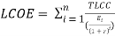
The levelized cost of energy, also known the levelized cost of electricity, or the levelized energy cost, is an economic assessment of the average total cost to build and operate a power-generating system over its lifetime divided by the total power generated of the system over that lifetime. LCOE is often used as an alternative to the average price that the power generating system must receive in a market to break even over its lifetime. LCOE is a first-order economic assessment of the cost competitiveness of an electricity-generating system that incorporates all costs over its lifetime accounting for the initial investment, the O&M cost, the cost of fuel, and the cost of capital.
The definition of LCOE is the cost that, if assigned to every unit of energy produced by the system over the analysis period, will equal the Total Life-Cycle Cost (TLCC) when discounted back to the base year [1][1],
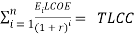 (1)
(1)
where discrete compounding is assumed, Ei is the amount of energy produced in year i, r is the WACC (or discount rate), and n is the number of years over which the LCOE is calculated. E in year i is calculated as,
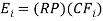 (2)
(2)
where RP is rated power, and CFiis the average capacity factor in year i. The TLCC in this model can be expressed as [11],
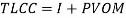 (3)
(3)
where I is the initial investment, and the Present Value of the total O&M costs (PVOM) is given by[11],
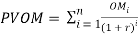 (4)
(4)
where OMi is the O&M costs in year i. LCOE is an equation that assigns a value for every unit produced during the given lifetime of a project. Traditionally, PPAs treat the contract length as the whole lifetime of the project, making short-term PPAs more expensive than long-term[11][12].
Since LCOE is by definition constant once calculated, it can be factored out of the summation in Equation (1) and the LCOE is given as,
 (5)
(5)
Although the denominator of Equation (5) appears to be discounting the energy (and some authors have characterize it as such), the discounting is actually a result of the algebra carried through from Equation (1) in which revenues were discounted (energy is not discounted, only cost can be discounted).
Based on the derivation of LCOE, the LCOE model must incorporate all financial parameters that contribute to the TLCC. Given this definition, this paper presents a model that includes PPA penalties in the TLCC.
Several LCOE models currently exist and are used to determine fair prices for wind energy. NREL uses SAM (System Advisor Model) to compute the LCOE using wind farm data for PPAs[7]. Equation 6shows the LCOE model used in SAM
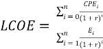 (6)
(6)
where CPEi is the cost to generate energy in year i and each parameter is given in the ith year.In the SAM model, the LCOE is calculated based on expected cash flows for O&M and capital expenditures. Although cash flow is important for determining the actual money spent and costs involved in a wind farm project, SAM does not recognize the implementation of penalties or tax credits in its wind LCOE model[7]. The SAM model does calculate a PPA price within its financial model that includes tax credits, but the PPA price is only a discounted value from the calculated LCOE and does not consider penalties.
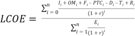
Similar to SAM, the most commonly used LCOE models do not include tax credits, production losses, or penalties. Some LCOE models, such as Equation (7)[8],
 (7)
(7)
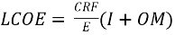
explicitly include the following costs: fuel cost (F), production tax credit (PTC), depreciation (D), tax levy (T), and royalties (R).[4] Equation (7) recognizes that the tax credits reduce costs, but it does not recognize PPA penalties as a cost. Other models, such as Equation (8)[6],
 (8)
(8)
where CRF is the capital recovery factor, consider the LCOE as a direct project cost and not the sum of TLCC of wind farms, which should include tax credits and PPA penalty costs in the TLCC. PPAs typically consider tax credits as a part of LCOE as seen in the Delmarva-Bluewater PPA[13] and explicitly in Equation (7). However, within PPAs, the LCOE calculation does not consider the cost of penalties in the life-cycle cost.
Current LCOE models do not consider all the cost parameters in a wind farm managed via a PPA. PPAs may define a maximum annual energy delivery quantity, a minimum annual energy delivery quantity, both of these limits, or neither. The energy delivery limits are cost parameters that are typically not considered in a conventional LCOE model. The terms generally follow the rule that after the maximum delivery is reached, energy will no longer is purchased by the Buyer, the energy will be sold at a reduced price, or it will be sold on the spot-market[14]. This is generally considered a cost/penalty for the Seller since they lose some value of the energy that is produced after the maximum delivery quantity is reached. Similarly, there is a direct cost/penalty in the minimum energy delivery defined in the PPA, as every unit of under-produced energy must be paid back at the agreed upon COE. We model the minimum delivery penalty based on the PacifiCorp draft PPA, which included the liquidated damages from output shortfall[15].
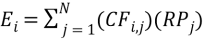
 In Fig. 1, the Maximum and Minimum energy limits demonstrate how the penalties are applied. Each year that the energy production is above or below the limits as shown in Fig. 1, the penalty is applied.
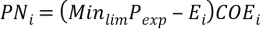
The new model reflects the costs of energy production that is above the maximum or below the minimum energy delivery limits. The model begins with an existing LCOE model (Equation (7)) and alters it to include the delivery penalties and tax credits.The cost for under-delivering energy (PN), is the difference between the energy that was generated and delivered (E) and the threshold for the minimum penalty (Minlim)based on expected energy production (Pexp). E is calculated by,
 (9)
(9)
where Eiis the sum of all the energy produced in the wind farm from N turbines in year i, CFi,j is the average capacity factor in year i for turbine j, and RPj is the rated power of turbine j. Using this calculation for energy, the production loss and the penalty from the minimum energy delivery limit can be calculated. PN is then calculated by,
 (10)
(10)
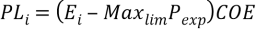
In Equation (10), Minlim is smallest fraction of expected energy production (Pexp) that the Buyer requires. The purpose of the minimum limit is for the benefit of the Buyer. The Buyer expects a minimum amount of energy to meet the demands of the consumers. If the energy does not meet the requirement, then the Buyer has to go to an outside source (e.g., the spot-market) and will may have to purchase energy at a higher cost, which the Buyer will require the Seller to compensate them for. Similarly, the production loss (PL) is the difference between the energy that was generated (E) in that year and the threshold for the maximum penalty (Maxlim) based on the Pexp.
 (1-PPAterm) (11)
In Equation (11), Maxlimis the largest fraction of expected energy production that the Buyer is willing to purchase. PN is only applied during the years that actual energy production is less than the quantity of energy determined by MinlimPexp,when Ei<MinlimPexp. PL is only applied when the energy produced exceeds the amount of energy determined by MaxlimPexp,when Ei>MaxlimPexp. PPAterm is a fraction that represents the type of penalty placed on the Seller after the maximum energy limit has been reached. In a PPA with no outside sell option the PPAterm has a value of0. When all the energy is purchased by the Buyer regardless of the limit the PPAtermis 1 and therefore PL is never applied.[5]
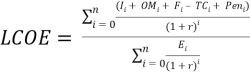
The LCOE model including all the unaccounted for cost variables that exist in PPAs is given by,
 (12)
(12)
where PL and PN are only included in the total penalty cost (Pen) when the calculated cost in either of those variables in a year is more than $0. In Equation (12) the sums in the numerator and denominator start at i = 0 under the assumption that the investment cost (Ii) comes from a depreciation schedule. In the case where the PPA allows for the Buyer to sell into the spot-market, the PL be a negative value. The Peni in year i is the sum of the production loss and the penalty cost,
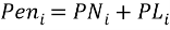 (13)
(13)
and the tax credit in year i (TCi) is given by,
 (14)
(14)
where all types of tax credits that can be applied to a wind farm are included (see nomenclature for specific tax credit contributions). Both of the Pen and the TC depend on the conditions imposed by the PPA.
A controlled study of wind farms was conducted to explore the effects of CF variation and energy delivery requirements on the LCOE. LCOEs were calculated based on four types of PPAs for farms with an annual CF that ranged in decreasing and increasing in fractions of 0 to 0.4 of the average CF around the average CF of 0.4. The four types of PPAs are: a PPA with just a minimum penalty, a PPA with just a maximum penalty where no energy can be bought above the limit, a PPA with just a maximum penalty where the energy is purchased at a fraction of 0.1 (PPAterm= 0.1) of the COE value for each unit of energy above the limit (the value of PPAterm= 0.1 was based on the Pakistan PPA[17]), and a PPA with just a maximum penalty where the energy above the maximum energy delivery limit has to be sold into the spot-market. Although the average CF = 0.4 is the same in all the cases considered, the COE for each wind farm is different since the LCOE differs for each wind farm due to the variations in CF. The costs and energy produced in each year varies, thus creating differences in the discounted total costs for each farm in the years that the CF varies. Each LCOE was calculated for a duration of 5 years. The following data was used to calculate the LCOE,
I = $1500 per installed kW[18]
OM = $0.01 per kWh produced[18]
F = $0[8]
TC = $0.05 per kWh sold[19]
r = 0.089 per year[20]
COE = Calculated LCOE from a PPA without penalties[21]
I, although shown as a single value, is a value that is depreciated over the lifetime of the wind farm and changes for every year i. The COE in a PPA is generally calculated from an LCOE that does not consider delivery penalties as a cost. For this reason, the cost calculated from penalties in the new model uses the calculated LCOE (for an individual wind farm) under a PPA without penalties as the COE. Pexpis calculated as the average annual expected energy production from a specific farm. In these cases the expected energy production is calculated using a CF of 0.4 for every year as Danish wind farms averaged 0.41 in 2012 and NREL has predicted that between 2005 and 2030, wind farms will be operating at capacity factors between 0.36 and 0.43[22]. Ei is calculated using a CF that is based on the variability around the average CF. The values of Minlim, Maxlim,and Ei, are then used to calculated penalties.
CF variation is the fraction of energy that is produced in year i that falls around the average CF of a project. Fig. 2 demonstrates this effect with two farms that have an average CF of 0.4 and a rated power of 2000 kW over 5 years. Wind farm 1 in this case has a CF variation of 0.05, this means that 0.05 more energy is produced in one year and 0.05 less is produced in another. Wind farm 2 in Fig. 2is similar as it portrays a CF variation of 0.15. The algorithm used in this study valued year 2 as the “unexpected” higher CF year and year 4 as the lower than “expected” CF year. It is possible to change the algorithm for other schedules of uncertainty that would yield different results and to make the schedule more complicated with random variations in random years.
In all of the LCOE verification tests, the LCOE follows a similar trend. Fig. 3 shows the results from a PPA with only a minimum energy delivery limit. In this case, as the fraction of expected energy production increases, more energy is likely to fall below the annual requirement, thus increasing the LCOE. The variation in CF determines the quantity below the minimum that the energy can fall to and how much the penalty cost will be to the Seller. The greater the variation, the more likely the LCOE will be effected by the minimum energy delivery limits.
Fig. 4shows a PPA where once the energy goes above the maximum annual energy delivery requirement that energy can be sold into the spot-market. The spot market is difficult to predict, therefore this study used spot-market prices from 2014 given by the EIA and used a Monte-Carlo simulation to randomly develop a normal distribution with a mean of $52.32 and a standard deviation of 38.75. Those values were then used to determine an expected value for the PPAtermfraction used in the produce the production loss calculation. In Fig. 4 the PPAterm = 1.1, which means that it was cheaper to sell into the spot-market then to sell to the Buyer under the PPA contract (i.e., “cheaper to sell” means more money for the Seller).[6] The results from Fig. 4 show that the LCOE drops when more energy is sold into the spot-market under these conditions. As the required energy fraction increased, only high variation farms have a lower LCOE because they are still producing above the maximum energy delivery limit and selling into the more profitable spot-market.
Fig. 5 and 6 show very similar trends for two different PPAs. Fig. 5contains results from a PPA with a PPAterm= 0.1 and Fig. 6contains results from a PPA with no outside sell option. Fig. 5allows for energy to be purchased after the maximum energy delivery limit has been reached, but only at PPAterm = 0.1 the value of the COE. This means that production loss is 0.9 of the COE for each unit of energy produced above the maximum energy delivery limit. Fig. 6 is similar because the production loss is the whole COE value for each unit of energy sold above the maximum energy delivery requirement because all the energy produced above the maximum limit cannot be sold, but is still being produced. Both figures show that as the Maxlimis increased, meaning that the maximum energy delivery requirement is increasing, less energy is being produced outside of the limit. Higher variations in the CF are more effected by the Maxlim than those with less variation. The only difference between Fig. 5and Fig. 6 is that in Fig. 5 the LCOE values are slightly lower than those in Fig. 6 This is due to the low value for the PPAterm.
A simulation was run to determine the resulting LCOEs from the four different PPA options. The first is a PPA with no energy delivery limits, where the energy is bought and sold as it is produced. The first type of PPA reflects a conventional LCOE where the PPA energy delivery limits are not applied. The second PPA has just a minimum delivery limit, the third has just a maximum delivery limits, and the fourth PPA has both delivery limits. Real data was collected from 7 different wind farms (Table 1[23]) that varied in the number of turbines, manufacturer, year built, rated power and country (Germany or Denmark). To simplify the differences in costs across the wind farms, the same cost variable values used in the model verification tests were used. The only difference in costs used from the model verification tests and the wind farm case study is that the wind farm case study uses a fixed COE for each farm at $0.25 per kWh, based on NREL’s highest expected COE[24]. These wind farms compared the four different PPA types with a fixed Maxlim = 0.75 and a Minlim = 0.52.[7] The LCOE of each turbine was calculated from the sum of LCOE costs at the end of 5 years. Fig. 7 shows the differences in the LCOEs based on the different annual energy delivery requirements and the selection of penalties that were applied. Each wind farm was given a number because the given data did not contain the name of the farms and only serial numbers for the turbines to identify that the turbines were a part of the same farm.
The results show that in most data sets, while using the same Maxlimand/or Minlim parameters, just having a maximum penalty produced LCOEs closest to the LCOEs with no penalties. The results also showed that LCOEs with both penalties or those with just minimum penalties produced higher LCOEs. Based on the results from the model verification tests, for wind farms with the same turbine types and year manufactured, it can be assumed that the different clusters of LCOEs are caused by the differences in CF. Lower CFs cause larger differences between a PPA with just a maximum penalty and a PPA with just a minimum penalty as produced by wind farm datasets 1 and 2. While datasets 4 and 7 show closer clusters of LCOE due to higher CFs that less frequently fall below the threshold for the minimum annual energy delivery limit, but more frequently have production loss by producing energy above the maximum annual energy delivery limit.

| Wind Farm
Dataset/ Manufacturer/ Rated Power< |
Cite This Work
To export a reference to this article please select a referencing stye below:
Related Services
View all


DMCA / Removal Request
If you are the original writer of this essay and no longer wish to have your work published on UKEssays.com then please click the following link to email our support team:
Request essay removal