Energy Losses in Pipes

ABSTRACT

The objective of this lab is to associate the loss of energy in a hydraulic system with the geometry of the pipe, that contains the fluid, while it is being transported from one location to another. Special considerations were given to major and minor energy losses. Friction was taken and treated as a major loss with respect to energy, while other factors such as expansions, contractions, pipe bends, pipe fittings and obstructions were considered as minor energy losses. The design of any hydraulic systems is governed by the understanding of these relations, and this experiment is carried out with the intention proving that there is a loss of energy specifically related to these factors. [4] The DMXL Base Unit ® in accordance with the DLM-6 ® cartridge were used to perform the experiment, using water as the medium of choice. The cartridge’s pressure transducers recorded the pressure differences at three locations of interest. The locations included a straight pipe section, a smooth 90° bend, and a sharp 90° right angle turn. For proper comparison, these results were all at the same length, of 70 mm. A total of 20 data points were tabulated, and used to calculate the loss of energy coefficients and head loss, for of all three sections. The results showed that there was a greater loss of energy with the sharp 90° right angle, followed by the smooth 90° bend and finally, the straight section had the least amount of energy loss. According to the principles of fluid mechanics, the assumption is that the highest loss of energy would correspond to the sharp 90° right angle bend. The results reinforced that assumption.

INTRODUCTION

In almost all hydraulic systems, it can be observed that there are energy losses with respect to friction and geometrical changes. The friction loss in pipes is due to the influence of the fluid’s viscosity near the surface of the surrounding pipe. The energy losses due to pressure changes can be seen in every part of a hydraulic system due to the expansions, contractions, bends in pipes, pipe fittings, and obstructions in the pipes. [2] This loss of energy is then transferred as heat.

Frictional losses in pipework are related to:

The complete acceptable pressure drop of the hydraulic system must be picked with care, as the power loss is a result of the pressure drop and system flow rate. There is an efficiency loss that must be adjusted for the cost of bigger fittings and hoses and pipework. The energy of no use is disseminated as heat energy in oil, which may prompt to cooling issues and condensing of the oil life. [1]

Pressure losses in pipework will rely on the fluid flow condition. There are three particular fluid

flow conditions:

As it can be seen in Figure 1, Laminar stream is the condition when the liquid particles travel easily in straight lines, the internal most liquid layer goes at the most elevated speed and the external most layer at the pipe surface doesn’t move. [2]

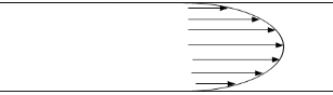
Figure 1. Laminar Flow [2]

Turbulent flow has unusual and disorderly liquid molecule movements, to such an extent that a comprehensive blending of the fluid happens, as appeared in Figure 2. A turbulent flow is generally not attractive, as the flow resistance increments and in this way the hydraulic losses increment. [3]

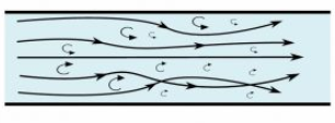
Figure 2. Turbulent Flow [3]

As shown in Figure 3, with turbulence in the focal point of the pipe, and laminar flow close to the edges, the transactional flow can be seen that it is a blend of the turbulent and laminar flow. [2]

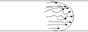
Figure 3. Transitional Flow [2]

Inside a pipe system, there are two sorts of losses. The first is a Major Loss and comprises of the head losses because of viscous impacts in straight fragments of pipe in the system. [5]

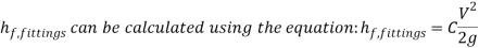
Which is referred to as h_(L major) and the equation follows as:

(1)

The second sort is a Minor Loss and is a form of losses produced inside segments of the pipe system other than the straight pipes themselves. [5]

Which is referred to as h_ (L minor) and the equation follows as:

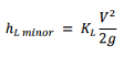(2)

The equation for head loss at a sudden expansion can be written as:

(3)

And expression for the head loss at a sudden contraction is as:

(4)

The head loss due to a bend can be shown by the expression as:

(5)

METHODOLOGY

Equipment and Materials List:

For the experiment, we used the Energy Losses in Hydraulic Systems cartridge on DLMX Base Unit ®. The DLMX is a teaching equipment that can be presented as one of the absolute best designed educating device that is utilized to teach students from various different subjects like Fluid Mechanics and Heat Transfer. The equipment includes a small battery operated, base unit, into which has one of the seven different cartridges is plugged. [3]

The base unit contains:

Experimental Apparatus:

According to the General Operating Instructions from the provided lab manual, the DLM-6 cartridge (Energy Losses in Hydraulic Systems) ® was installed as shown below in Figure 4, with a filled Base Unit and powered on. The flow rate was adjusted using the knob on the Base Unit. The flow rate and corresponding differential pressure readings across the straight pipe, smooth bend and sharp bend sections appeared on the output screen.

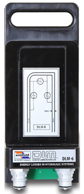
Figure 4. DLM-6 cartridge (Energy Losses in Hydraulic Systems) [3]

The cartridges have the particular instrumentation required for the specific demonstration and contain an experimental representation of the topic. The base unit involves a round, clear acrylic water reservoir, mounted on a powerful vacuum shaped ABS plastic plinth, shown below in Figure (#). Under the plinth is a pump with a variable speed control, battery, flow meter, the electrical control hardware, and level sensor [6].

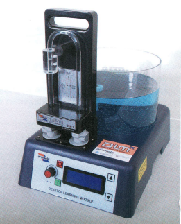
Figure (5) Energy Losses in Hydraulic Systems cartridge on DLMX Base Unit [3]

Experimental Procedure:

To commensurate our lab, we referred to “Filling Pressure Transducer Tubes” section as we powered on the machine. We then installed the DLM-6 cartridge (Energy Losses in Hydraulic Systems) ® into the Base Unit filled with water and ensured that all pressure readings are at zero flow rate. We can read the flow rate and pressure drop at that moment is given if we scrolled down on the display on the machine. Next, we checked for the possible maximum flow rate. From there we were able to get an estimate of the increment differences needed for each reading. The flow rate was set to ~ 1 L/min and increased in approximately equal increments until the maximum flow rate was achieved. And then the pressure drop was obtained and recorded. Steps were repeated until Experimental DLMX ® data table is completed.

RESULTS

Table 1 shows the data points recorded from different runs of fluid flowing through ΔP – Straight, ΔP – Smooth, and ΔP – RA Bend.

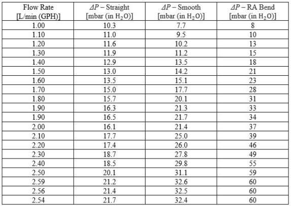
Table 1. Data points recorded from the experiment.

Dimension & Constants:

Square pipe width = 4 mm

Smooth bend radius = 8 mm

(to channel center)

Distance between pressure taps:

Straight section: 70 mm

Smooth bend section: 70 mm

Sharp bend section: 70

Ç‚RA = right angle bend

Velocity:

In Table 2, we found the Velocity by using the equation of Flow rate,

Area: (area = 0.004*0.004 =0.000016 m²); Q: Flow rate

(6)

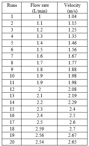
Table 2. Velocity obtained from different runs.

Headloss:

Head loss for straight, smooth and right angle pipe are shown below in Table 3:

We used Pascal’s Law to calculate the loss coefficient.

This can be found by using equation of:

H_L = (7)

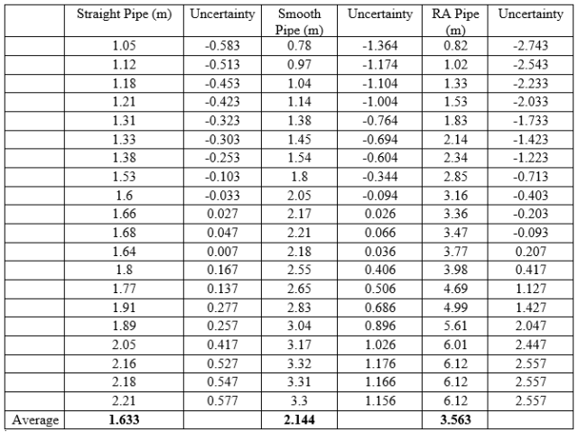
Table 3. Head loss for straight, smooth and right angle pipe

Loss Coefficient:

K smooth =289.30, k RA= 267.48, f Straight= 1.461*10^-4,

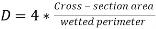
As we know that hydraulic diameter,

(8)

(9)

therefore,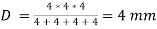

The values below are derived from basic equation of Head loss,

H_L = {This same equation is used for straight pipes}

{This same equation is used for smooth and RA pipes}

In the above equations f and K are the loss coefficients.

Loss coefficients for straight, smooth and right angle pipes are shown below:

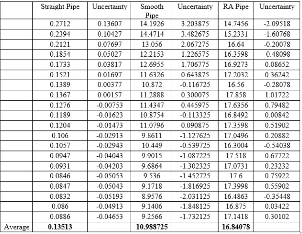
Table 4. Loss coefficients of Straight, Smooth, and RA Bend Pipe.

DISCUSSION

In order to obtain the pressure difference in a circular pipe it is possible to reduce the energy equation as follows.

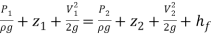(10)

(11)

Where,

á‘­ = Density of fluid, g = gravity, h = height, P = pressure, V = average velocity, z = elevation and

This reduction is applicable when the cross-sectional area as well as the elevation are equal.

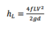
For circular channels, the head loss due to flow can be obtained using the equation below.

(12)

Where,

f = Stanton friction factor, L = length of circular channel, D = diameter, V = average velocity and g = gravity.

In contrast to circular channels, the energy equation can also be used to obtain the pressure difference in noncircular channels as follows.

(13)

However, in noncircular channels, the head loss due to flow can be obtained using the equation

(14)

Where,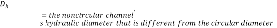

(15)

Moreover, the friction factor for non-circular channels is a function of the roughness factor divided by the hydraulic radius and the Reynold’s number.

(16)

For noncircular channels, the Reynolds number is also calculated using the hydraulic diameter as follows.

(17)

It is possible to measure pressure losses arising from fittings to the piping system using the DLMX fluid mechanics cartridge fitted with differential pressure transducers that connected to pressure taps which registers the difference in pressure related to the flow.

The pressure difference can be evaluated using the energy equation that includes major friction losses due to fittings on the piping system as follows.

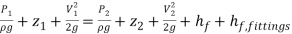(18)

For the cartridge, the energy balance equation begins as follows below.

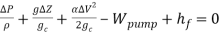(19)

Considering the cartridge as a closed system the energy balance equation reduces as follows below.

(20)

Physically, represents the pressure losses per unit mass of water in the cartridge. On the other hand, represents the differences in pressure at the three points of interest associated with flow. The hierarchy of pressure difference starting from the least pressure difference to the highest is as follows below.

The pressure drop at the right-angled bend can be calculated using from the energy balance equation below.

(21)

Because there is no change in diameter throughout the length of the bend, no change in elevation, as well as no change in elevation, the energy balance equation reduces to.

(22)

The loss coefficient is a dimensionless coefficient derived from dividing the head loss by as follows below.

(23)

Therefore,

Finally, to calculate the required pressure losses in the bend the equation above reduces as follows below.

(24)

At the straight portion of the pipe, the pressure drop equation reduces as follows below.

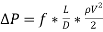(25)

Where f=the friction coefficient, D=diameter of the pipe and L= the length of the pipe.

In order to find the length of straight pipe that would be sufficient to generate the same amount of pressure drop at the right-angled bend the pressure drops have to be made equal as follows below.

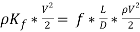(26)

The length of the pipe then reduces to the formula below.

(27)

It is possible to determine the loss coefficient graphically from the experimental values by creating a graph of the head loss vs dynamic head.

(28)

Where and = dynamic head, the loss coefficient

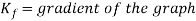
Figure 6. Head loss vs Dynamic Head

CONCLUSION

The goals of this lab was to measure the head losses through straight, smooth, and sharp- bend pipe fittings and then use these measurements to estimate the loss of energy coefficients for each transition or fitting. For the experiment, the DML-6 ® cartridge (Energy Losses in Hydraulic Systems) was used with the DLMX Base Unit ®, using water as the fluid of choice. The flow rate and corresponding differential pressure readings across the straight pipe, smooth bend and sharp bend sections were all recorded. A total of 20 data points were collected. The collected datas were used to calculate the head losses and loss of energy coefficients for all three sections. The results show that the pressure difference in the right-angle bend is higher than smooth bend, and pressure difference in smooth is higher than the straight bend pipes. Also, the average head loss of a right-angle pipe, 1.633, is certainly higher than average head loss of the smooth, 2.144, and straight, 1.633. Furthermore, the average loss coefficient of right angle pipe, 16.84078, was also higher than smooth, 10.988725, and straight, 0.13513, pipes. Uncertainty analysis indicate that one possible source of error came from the pressure readings. The pressure readings at the reference point for each component and each flow was some value greater than zero, but the problem with this was that all the reference point readings should have been zero regardless of the set up. The reason for this difference is still unknown, however the doubt is that there was a problem with the machine’s manometer. The lesson learned with this experiment was the energy losses in pipes due to different fittings. The experiment was quite interesting, yet this hands-on approach lesson will help us succeed in the real engineering world as well.

REFERENCES

[1] Bruce Roy, Munson, T. H. Okiishi and Donald F. Young. Fundamentals of Fluid Mechanics. Hoboken, NJ: J. Wiley & Sons, 2009.

[2] Smith, W.F., “Turbulent and Laminar Flow in Pipes, with the Particular Reference to the Transition between the Straight, Smooth and Rough Pipe Laws,” J. Inst. Civ. Eng. Lond., vol.11, pp. 148-178, 1979-78.

[3] DLMX Base Unit and DLM-6 Energy Losses in Hydraulic Systems. (2017, February 28). Retrieved from http://discoverarmfield.com/en/products/view/dlmx/desktop-learning-modules

[3] Hibbeler, R. C. “10.2 Losses Occurring from Pipe Fittings and Laminar, Turbulent, and Transitions.” Fluid Mechanics. N.p.: Pearson Prentice Hall, 2015. 578-46. Print.

[4] “Fluid Flow through between Pipes.” Pump-House, University of South Carolina, Columbia (2007): n. pag. Web. http://www.cs.cdu.edu.au/home-page/jayitroy/eng477/sect10.pdf – pg. 47

[5] “Head Loss Coefficients of Major and Minor.” Vano Engineering. N.p., 13 Dec. 2014. Web. 20 Jan. 2015.

[6] Shukla. S.K.,” Indian Journal of Applied Research, of various different flow rates, vol. 7, no. 7, pp. 313-377, April. 2015.

[7] Donald, James C., M. F. Sherif, and V. P. Kumar. “8.4 Minor and Major Losses in Pipes.” Elementary Hydraulics. Mason, OH: Cengage Learning, 2004. 257-78. Print.

[8] John Ray, W.F., 1947, “Turbulent Flow in Pipes with Particular reference to the Transition

Region between the Smooth and Rough Pipe Laws“, J. Institution. of Civil Engr Dept., I7, pp 178-167.

APPENDIX A

We learned how different pipe fittings results in energy losses in pipes. Although it was quite difficult to do all the calculations, plus the presence of uncertainty created a doubt on the result, our team found this lab very interesting. The results were also close to the expected outcome.

APPENDIX B

APPENDIX C

It should be noted that when using Bernoulli’s equation, one must take into consideration the height of a pipe. The data that was used in the calculations was processed without that consideration. The manufacturer of the unit explains that the pressure transducers inside the DLM-6 ® cartridge do not measure hydrostatic pressures between the taps, when the tubes are filled with water. As it can be seen in the image below the device is filled with water, but the water is not in motion. The levels of the manometer tubes are the same, regardless of the vertical setup. With the same concept in mind, it is clear to see that the pressure transducers will also fail to measure any pressure change with respect to gravity.