Compression Techniques used for Medical Image

1.1 Introduction

Image compression is an important research issue over the last years. A several techniques and methods have been presented to achieve common goals to alter the representation of information of the image sufficiently well with less data size and high compression rates. These techniques can be classified into two categories, lossless and lossy compression techniques. Lossless techniques are applied when data are critical and loss of information is not acceptable such as Huffman encoding, Run Length Encoding (RLE), Lempel-Ziv-Welch coding (LZW) and Area coding. Hence, many medical images should be compressed by lossless techniques. On the other hand, Lossy compression techniques such as Predictive Coding (PC), Discrete Wavelet Transform (DWT), Discrete Cosine Transform (DCT) and Vector Quantization (VQ) more efficient in terms of storage and transmission needs but there is no warranty that they can preserve the characteristics needed in medical image processing and diagnosis [1-2].

Data compression is the process that transform data files into smaller ones this process is effective for storage and transmission. It presents the information in a digital form as binary sequences which hold spatial and statistical redundancy. The relatively high cost of storage and transmission makes data compression worthy. Compression is considered necessary and essential key for creating image files with manageable and transmittable sizes [3].

The basic goal of image compression is to reduce the bit rate of an image to decrease the capacity of the channel or digital storage memory requirements; while maintaining the important information in the image [4]. The bit rate is measured in bits per pixel (bpp). Almost all methods of image compression are based on two fundamental principles:

1. The first principle is to remove the redundancy or the duplication from the image. This approach is called redundancy reduction.
2. The second principle is to remove parts or details of the image that will not be noticed by the user. This approach is called irrelevancy reduction.

Image compression methods are based on either redundancy reduction or irrelevancy reduction separately while most compression methods exploit both. While in other methods they cannot be easily separated [2]. Several image compression techniques encode transformed image data instead of the original images [5]-[6].

In this thesis, an approach is developed to enhance the performance of Huffman compression coding a new hybrid lossless image compression technique that combines between lossless and lossy compression which named LPC-DWT-Huffman (LPCDH) technique is proposed to maximize compression so that threefold compression can be obtained. The image firstly passed through the LPC transformation. The waveform transformation is then applied to the LPC output. Finally, the wavelet coefficients are encoded by the Huffman coding. Compared with both Huffman, LPC- Huffman and DWT-Huffman (DH) techniques; our new model is as maximum compression ratio as that before. However, this is still needed for more work especially with the advancement of medical imaging systems offering high resolution and video recording. Medical images come in the front of diagnostic, treatment and fellow up of different diseases. Therefore, nowadays, many hospitals around the world are routinely using medical image processing and compression tools.

1.1.1 Motivations

Most hospitals store medical image data in digital form using picture archiving and communication systems due to extensive digitization of data and increasing telemedicine use. However, the need for data storage capacity and transmission bandwidth continues to exceed the capability of available technologies. Medical image processing and compression have become an important tool for diagnosis and treatment of many diseases so we need a hybrid technique to compress medical image without any loss in image information which important for medical diagnosis.

1.1.2 Contributions

Image compression plays a critical role in telemedicine. It is desired that either single images or sequences of images be transmitted over computer networks at large distances that they could be used in a multitude of purposes. The main contribution of the research is aim to compress medical image to be small size, reliable, improved and fast to facilitate medical diagnosis performed by many medical centers.

1.2 Thesis Organization

The thesis is organized into six chapters, as following:

Chapter 2 Describes the basic background on the image compression technique including lossless and lossy methods and describes the types of medical images

Chapter 3 Provides a literature survey for medical image compression.

Chapter 4 Describes LPC-DWT-Huffman (proposed methods) algorithm implementation. The objective is to achieve a reasonable compression ratio as well as better quality of reproduction of image with a low power consumption.

Chapter 5 Provides simulation results of compression of several medical images and compare it with other methods using several metrics.

Chapter 6 Provides some drawn conclusions about this work and some suggestions for the future work.

Appendix A Provides Huffman example and comparison between the methods for the last years.

Appendix B Provides the Matlab Codes

Appendix C Provides various medical image compression using LPCDH.

1.3 Introduction

Image compression is the process of obtaining a compact representation of an image while maintaining all the necessary information important for medical diagnosis. The target of the Image compression is to reduce the image size in bytes without effects on the quality of the image. The decrease in image size permits images to save memory space. The image compression methods are generally categorized into two central types: Lossless and Lossy methods. The major objective of each type is to rebuild the original image from the compressed one without affecting any of its numerical or physical values [7].

Lossless compression also called noiseless coding that the original image can perfectly recover each individual pixel value from the compressed (encoded) image but have low compression rate. Lossless compression methods are often based on redundancy reduction which uses statistical decomposition techniques to eliminate or remove the redundancy (duplication) in the original image. Lossless Image coding is also important in applications where no information loss is allowed during compression. Due to the cost, it is used only for a few applications with stringent requirements such as medical imaging [8-9].

In lossy compression techniques there are a slight loss of data but high compression ratio. The original and reconstructed images are not perfectly matched. However, practically near to each other, this difference is represented as a noise. Data loss may be unacceptable in many applications so that it must be lossless. In medical images compression that use lossless techniques do not give enough advantages in transmission and storage and the compression that use lossy techniques may lose critical data required for diagnosis [10]. This thesis presents a combination of lossy and lossless compression to get high compressed image without data loss.

1.4 Lossless Compression

If the data have been lossless compressed, the original data can be exactly reconstructed from the compressed data. This is generally used for many applications that cannot allow any variations between the original and reconstructed data. The types of lossless compression can be analyzed in Figure 2.1.

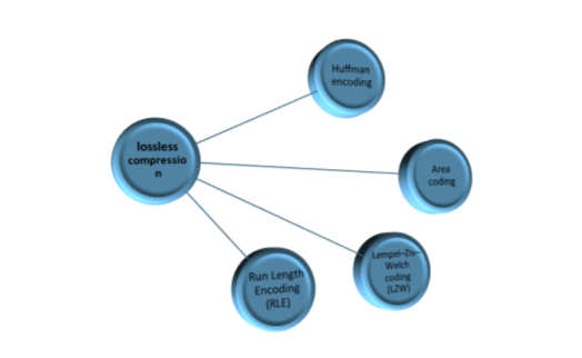
Figure 2.1: lossless compression

1. Run Length Encoding

Run length encoding, also called recurrence coding, is one of the simplest lossless data compression algorithms. It is based on the idea of encoding a consecutive occurrence of the same symbol. It is effective for data sets that are consist of long sequences of a single repeated character [50]. This is performed by replacing a series of repeated symbols with a count and the symbol. That is, RLE finds the number of repeated symbols in the input image and replaces them with two-byte code. The first byte for the number and the second one is for the symbol. For a simple illustrative example, the string ‘AAAAAABBBBCCCCC’ is encoded as ‘A6B4C5’; that saves nine bytes (i.e. compression ratio =15/6=5/2). However in some cases there is no much consecutive repeation which reduces the compression ratio. An illustrative example, the original data “12000131415000000900”, the RLE encodes it to “120313141506902” (i.e. compression ratio =20/15=4/3). Moreover if the data is random the RLE may fail to achieve any compression ratio [30]-[49].

2. Huffman encoding

It is the most popular lossless compression technique for removing coding redundancy. The Huffman encoding starts with computing the probability of each symbol in the image. These symbols probabilities are sorted in a descending order creating leaf nodes of a tree. The Huffman code is designed by merging the lowest probable symbols producing a new probable, this process is continued until only two probabilities of two last symbols are left. The code tree is obtained and Huffman codes are formed from labelling the tree branch with 0 and 1 [9]. The Huffman codes for each symbol is obtained by reading the branch digits sequentially from the root node to the leaf. Huffman code procedure is based on the following three observations:

1) More frequently(higher probability) occurred symbols will have shorter code words than symbol that occur less frequently.

2) The two symbols that occur least frequently will have the same length code.

3) The Huffman codes are variable length code and prefix code.

For more indication Huffman example is presented in details in Appendix (A-I).

The entropy (H) describes the possible compression for the image in bit per pixel. It must be noted that, there aren’t any possible compression ratio smaller than entropy. The entropy of any image is calculated as the average information probability [12].

(2.1)

Where P_k is the probability of symbols, k is the intensity value, and L is the number of intensity values used to present image.

The average code length is given by the sum of product of probability of the symbol and number of bits used to encode it. More information can be founded in [13-14] and the Huffman code efficiency is calculated as

(2.2)

3. LZW coding

LZW (Lempel- Ziv – Welch) is given by J. Ziv and A. Lempel in 1977 [51].T. Welch’s refinements to the algorithm were published in 1984 [52]. LZW compression replaces strings of characters with single codes. It does not do any analysis of the input text. But, it adds every new string of characters to a table of strings. Compression occurs when the output is a single code instead of a string of characters.

LZW is a dictionary based coding which can be static or dynamic. In static coding, dictionary is fixed during the encoding and decoding processes. In dynamic coding, the dictionary is updated. LZW is widely used in computer industry and it is implemented as compress command on UNIX [30]. The output code of that the LZW algorithm can be any arbitrary length, but it must have more bits than a single character. The first 256 codes are by default assigned to the standard character set. The remaining codes are assigned to strings as the algorithm proceeds. There are three best-known applications of LZW: UNIX compress (file compression), GIF image compression, and V.42 bits (compression over Modems) [50].

4. Area coding

Area coding is an enhanced form of RLE. This is more advance than the other lossless methods. The algorithms of area coding find rectangular regions with the same properties. These regions are coded into a specific form as an element with two points and a certain structure. This coding can be highly effective but it has the problem of a nonlinear method, which cannot be designed in hardware [9].

1.5 Lossy Compression

Lossy Compression techniques deliver greater compression percentages than lossless ones. But there are some loss of information, and the data cannot be reconstructed exactly. In some applications, exact reconstruction is not necessary. The lossy compression methods are given in Figure 2.2. In the following subsections, several Lossy compression techniques are reviewed:

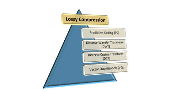Figure 2.2: lossy compression

1. Discrete Wavelet Transform (DWT)

Wavelet analysis have been known as an efficient approach to representing data (signal or image). The Discrete Wavelet Transform (DWT) depends on filtering the image with high-pass filter and low-pass filter.in the first stage The image is filtered row by row (horizontal direction) with two filters and and down sampling (keep the even indexed column) every samples at the filter outputs. This produces two DWT coefficients each of size N Ã-N/2. In the second stage, the DWT coefficients of the filter are filtered column by column (vertical direction) with the same two filters and keep the even indexed row and subsampled to give two other sets of DWT coefficients of each size N/2Ã-N/2. The output is defined by approximation and detailed coefficients as shown in Figure 2.3.

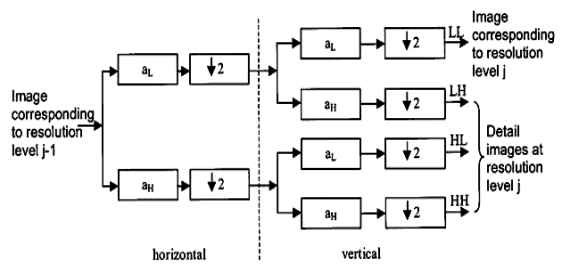
Figure 2.3: filter stage in 2D DWT [15].

LL coefficients: low-pass in the horizontal direction and lowpass in the vertical direction.

HL coefficients: high-pass in the horizontal direction and lowpass in the vertical direction, thus follow horizontal edges more than vertical edges.

LH coefficients: high-pass in the vertical direction and low-pass in the horizontal direction, thus follow vertical edges than horizontal edges.

HH coefficients: high-pass in the horizontal direction and high-pass in the vertical direction, thus preserve diagonal edges.

Figure 2.4 show the LL, HL, LH, and HH when one level wavelet is applied to brain image. It is noticed that The LL contains, furthermore all information about the image while the size is quarter of original image size if we disregard the HL, LH, and HH three detailed coefficients shows horizontal, vertical and diagonal details. The Compression ratio increases when the number of wavelet coefficients that are equal zeroes increase. This implies that one level wavelet can provide compression ratio of four [16].

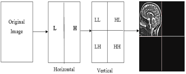
Figure 2.4: Wavelet Decomposition applied on a brain image.

The Discrete Wavelet Transform (DWT) of a sequence consists of two series expansions, one is to the approximation and the other to the details of the sequence. The formal definition of DWT of an N-point sequence x [n], 0 ≤ n ≤ N − 1 is given by [17]:

(2.3)

(2.4)

(2.5)

Where Q (n₁ ,n₂) is approximated signal, E(n₁ ,n₂) is an image, W_Q (j,k₁,k₂) is the approximation DWT and W_µ (j,k₁,k₂) is the detailed DWT where i represent the direction index (vertical V, horizontal H, diagonal D) [18].

To reconstruct back the original image from the LL (cA), HL (cD^(h)), LH (cD^(v)), and HH (cD^(d)) coefficients, the inverse 2D DWT (IDWT) is applied as shown in Figure 2.5.

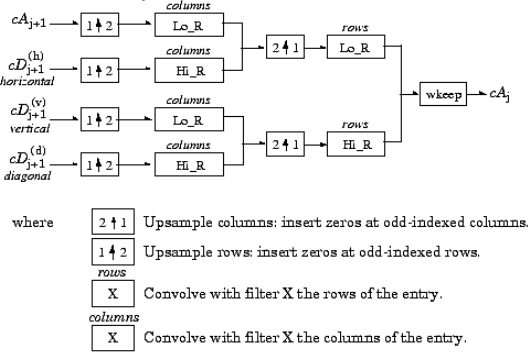
Figure 2.5: one level inverse 2D-DWT [19].

The equation of IDWT that reconstruct the image E () is given by [18]:

(2.6)

DWT has different families such as Haar and Daupachies (db) the compression ratio can vary from wavelet type to another depending which one can represented the signal in fewer number coefficients.

2. Predictive Coding (PC)

The main component of the predictive coding method is the “Predictor” which exists in both encoder and decoder. The encoder computes the predicted value for a pixel, denote xˆ(n), based on the known pixel values of its neighboring pixels. The residual error, which is the difference value between the actual value of the current pixel x (n) and x ˆ(n) the predicted one. This is computed for all pixels. The residual errors are then encoded by any encoding scheme to generate a compressed data stream [21]. The residual errors must be small to achieve high compression ratio.

e (n) = x (n) – xˆ(n)(2.7)

e (n) =x(n) – 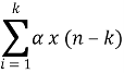(2.8)

Where k is the pixel order and α is a value between 0 and 1 [20].

The decoder also computes the predicted value of the current pixel xˆ (n) based on the previously decoded color values of neighboring pixels using the same method as the encoder. The decoder decodes the residual error for the current pixel and performs the inverse operation to restore the value of the current pixel [21].

x (n) = e (n) + xˆ (n)(2.9)

1. Linear predictive coding (LPC)

The techniques of linear prediction have been applied with great success in many problems of speech processing. The success in processing speech signals suggests that similar techniques might be useful in modelling and coding of 2-D image signals. Due to the extensive computation required for its implementation in two dimensions, only the simplest forms of linear prediction have received much attention in image coding [22]. The schemes of one dimensional predictors make predictions based only on the value of the previous pixel on the current line as shown in equation.

Z = X – D(2.10)

Where Z denotes as output of predictor and X is the current pixel and D is the adjacent pixel.

The two dimensional prediction scheme based on the values of previous pixels in a left-to-right, top-to-bottom scan of an image. In Figure 2.6 X denotes the current pixel and A, B, C and D are the adjacent pixels. If the current pixel is the top leftmost one, then there is no prediction since there are no adjacent pixels and no prior information for prediction [21].

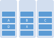
Figure 2.6: Neighbor pixels for predicting

Z = x – (B + D)(2.11)

Then, the residual error (E), which is the difference between the actual value of the current pixel (X) and the predicted one (Z) is given by the following equation.

E = X – Z(2.12)

3. Discrete Cosine Transform (DCT)

The Discrete Cosine Transform (DCT) was first proposed by N. Ahmed [57]. It has been more and more important in recent years [55]. The DCT is similar to the discrete Fourier transform that transforms a signal or image from the spatial domain to the frequency domain as shown in Figure 2.7.

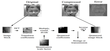
Figure 2.7: Image transformation from the spatial domain to the frequency domain [55].

DCT represents a finite series of data points as a sum of harmonics cosine functions. DCTs representation have been used for numerous data processing applications, such as lossy coding of audio signal and images. It has been found that small number of DCT coefficients are capable of representing large sequence of raw data. This transform has been widely used in signal processing of image data, especially in coding for compression for its near-optimal performance. The discrete cosine transform helps to separate the image into spectral sub-bands of differing importance with respect to the image’s visual quality [55]. The use of cosine is much more efficient than sine functions in image compression since this cosine function is capable of representing edges and boundary. As described below, fewer coefficients are needed to approximate and represent a typical signal.

The Two-dimensional DCT is useful in the analysis of two-dimensional (2D) signals such as images. We say that the 2D DCT is separable in the two dimensions. It is computed in a simple way: The 1D DCT is applied to each row of an image, s, and then to each column of the result.

Thus, the transform of the image s(x, y) is given by [55],

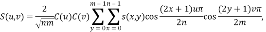(2.13)

where. (n x m) is the size of the block that the DCT is applied on. Equation (2.3) calculates one entry (u, v) of the transformed image from the pixel values of the original image matrix [55]. Where u and v are the sample in the frequency domain.

DCT is widely used especially for image compression for encoding and decoding, at encoding process image divided into N x N blocks after that DCT performed to each block. In practice JPEG compression uses DCT with a block of 8×8. Quantization applied to DCT coefficient to compress the blocks so selecting any quantization method effect on compression value. Compressed blocks are saved in a storage memory with significantly space reduction. In decoding process, compressed blocks are loaded which de-quantized with reverse the quantization process. Inverse DCT was applied on each block and merging blocks into an image which is similar to original one [56].

4. Vector Quantization

Vector Quantization (VQ) is a lossy compression method. It uses a codebook containing pixel patterns with corresponding indexes on each of them. The main idea of VQ is to represent arrays of pixels by an index in the codebook. In this way, compression is achieved because the size of the index is usually a small fraction of that of the block of pixels. The image is subdivided into blocks, typically of a fixed size of nÃ-n pixels. For each block, the nearest codebook entry under the distance metric is found and the ordinal number of the entry is transmitted. On reconstruction, the same codebook is used and a simple look-up operation is performed to produce the reconstructed image [53].

The main advantages of VQ are the simplicity of its idea and the possible efficient implementation of the decoder. Moreover, VQ is theoretically an efficient method for image compression, and superior performance will be gained for large vectors. However, in order to use large vectors, VQ becomes complex and requires many computational resources (e.g. memory, computations per pixel) in order to efficiently construct and search a codebook. More research on reducing this complexity has to be done in order to make VQ a practical image compression method with superior quality [50].

Learning Vector Quantization is a supervised learning algorithm which can be used to modify the codebook if a set of labeled training data is available [13]. For an input vector x, let the nearest code-word index be i and let j be the class label for the input vector. The learning-rate parameter is initialized to 0.1 and then decreases monotonically with each iteration. After a suitable number of iterations, the codebook typically converges and the training is terminated. The main drawback of the conventional VQ coding is the computational load needed during the encoding stage as an exhaustive search is required through the entire codebook for each input vector. An alternative approach is to cascade a number of encoders in a hierarchical manner that trades off accuracy and speed of encoding [14], [54].

1.6 Medical Image Types

Medical imaging techniques allow doctors and researchers to view activities or problems within the human body, without invasive neurosurgery. There are a number of accepted and safe imaging techniques such as X-rays, Magnetic resonance imaging (MRI), Computed tomography (CT), Positron Emission Tomography (PET) and Electroencephalography (EEG) [23-24].

1.7 Conclusion

In this chapter many compression techniques used for medical image have discussed. There are several types of medical images such as X-rays, Magnetic resonance imaging (MRI), Computed tomography (CT), Positron Emission Tomography (PET) and Electroencephalography (EEG). Image compression has two categories lossy and lossless compression. Lossless compression such as Run Length Encoding, Huffman Encoding Lempel-Ziv-Welch, and Area Coding. Lossy compression such as Predictive Coding (PC), Discrete Wavelet Transform (DWT), Discrete Cosine Transform (DCT), and Vector Quantization (VQ).Several compression techniques already present a better techniques which are faster, more accurate, more memory efficient and simpler to use. These methods will be discussed in the next chapter.