Change Detection Techniques of Remote Sensing Imageries
| ✅ Paper Type: Free Essay | ✅ Subject: Engineering |
| ✅ Wordcount: 3218 words | ✅ Published: 31 Aug 2017 |
1.1 Introduction
Over the past years, academics have suggested enormous numbers of change detection techniques of remote sensing imageries and classified them from a different point of views [28]. These techniques depend on the assumption of spatial independence among pixels. This assumption is valid only for low, medium and high-resolution images but insufficient for VHR images [1]. This chapter presents the concept, implementation, and assessment of seven change detection techniques using low, medium and high-resolution ORSI. The rest of this chapter is organized into eight sections. Section 3.2 presents a brief description of the study areas. Section 3.3 describes the dataset characteristics of the study areas (Sharm El-Sheikh city and Mahalla al-kubra city – Egypt). Section 3.4 presents the pre-processing performed on the image dataset before change detection process. Section 3.5 provides the accuracy assessment measures used for evaluation of the change detection process. Section 3.6 illustrates the concepts of the selected seven change detection techniques. These techniques are post-classification, direct multi-date classification (DMDC), image differencing (ID), image rationing (IR), image symmetric relative difference (ISRD), change vector analysis (CVA), and principal component differencing (PCD). Section 3.7 presents the experimental work. It explains the Implementation and accuracy assessment of applying the selected change detection techniques on an image dataset of Sharm El-Sheikh city- Egypt. Section 3.8 presents the application of “post-classification” change detection technique on an image dataset of El-Mahalla El-kubra City-Egypt to detect the urban expansion over the agricultural area through the period from 2010 to 2015. Finally, section 3.9 gives the chapter summary.
1.2 The study areas
In this chapter, two study areas are selected for the application of the selected change detection techniques. The first area is a part of Sharm el-Sheikh city. It is located on the southern landfill of the Sinai Peninsula, in the South Sinai Governorate, Egypt, on the coastal bar along the Red Sea as shown in figure (3.1).
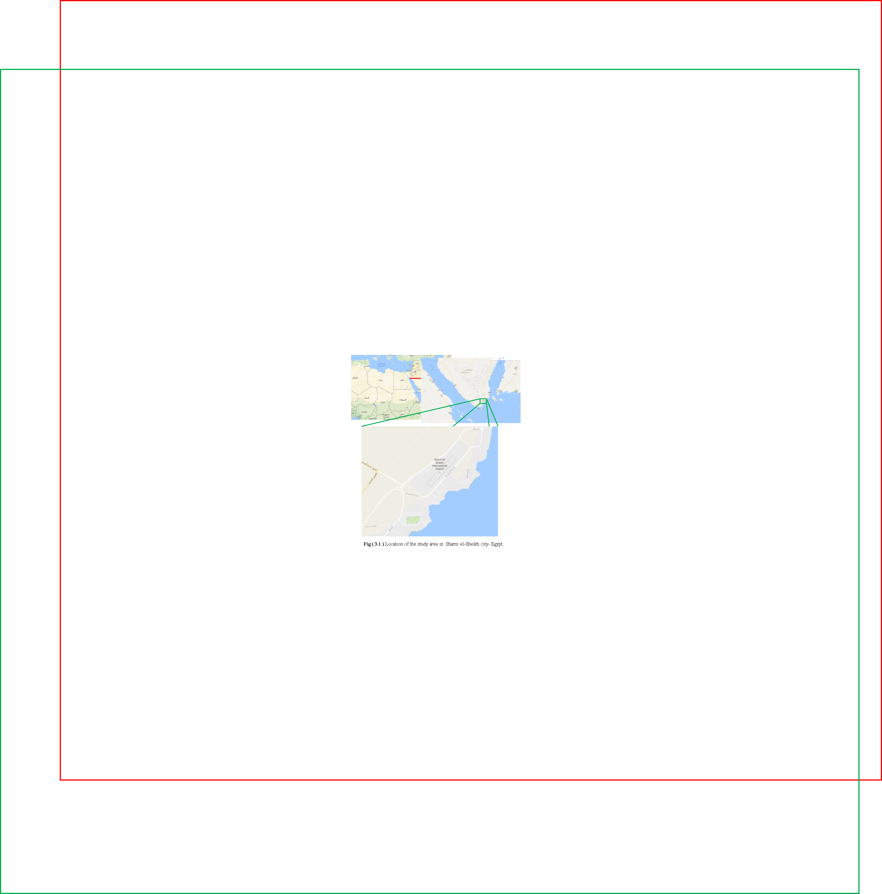
Its population is approximately 73,000 as of 2015 [62]. Sharm El Sheikh is the administrative hub of Egypt’s South Sinai Governorate, which includes the smaller coastal towns of Dahab and Nuweiba as well as the mountainous interior, St. Catherine and Mount Sinai. Today the city is a holiday resort and significant center for tourism in Egypt. The selected area is about 12.5 Km2.
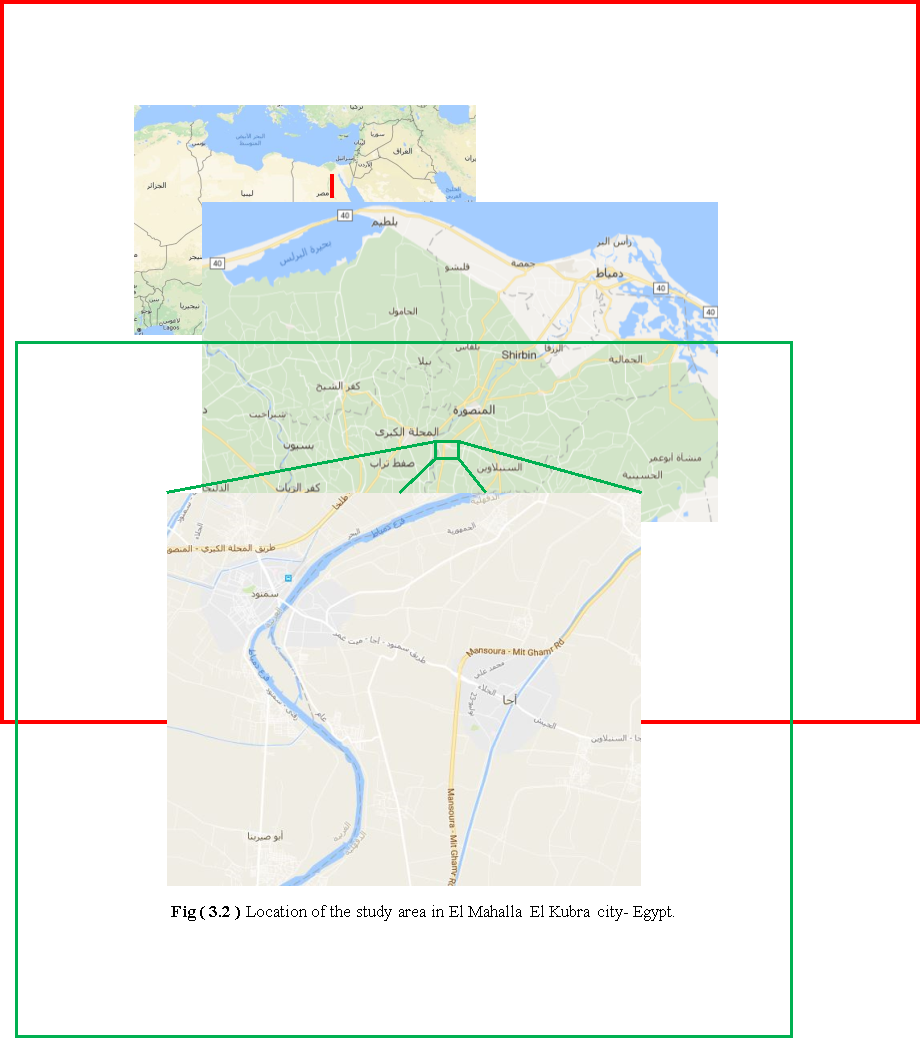
The second study area is a village belongs to El Mahalla El Kubra city. El Mahalla El Kubra is a large industrial and agricultural city in Egypt, located in the middle of the Nile Delta on the western bank of the Damietta Branch tributary, as shown in figure (3.2). The city is known for its textile industry. It is the largest city of the Gharbia Governorate and the second largest in the Nile Delta [63]. The selected area is about 38 Km2.
1.3 Images datasets of the study areas
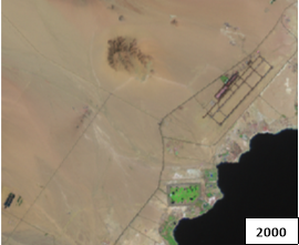
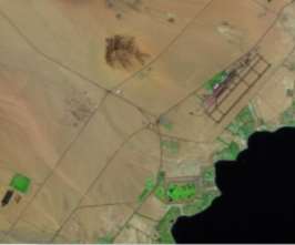
In this chapter, two datasets are used. The first dataset consists of two images of Sham el-Sheikh city acquired by Landsat 7 at 2000 and 2010 respectively as shown in figure (3.3). Area of the image lies between Lat. 28 0 37.0091 N, Lon. 34 17 56.3381 E and Lat. 27 57 20.8804 N, Lon. 34 24 43.6080 E. Table (3.1) summarizes the characteristic of these images.
|
No |
Spatial resolution |
Radiometric resolution |
Number of bands |
Acquisition date |
Size [pixels] |
Area [km2] |
|
|
Width |
Height |
||||||
|
1 |
30 m |
8 bits |
3 |
2000 |
382 |
364 |
12.5143 |
|
2 |
30 m |
8 bits |
3 |
2010 |
382 |
364 |
12.5143 |
|
|
|
|
(a) |
(b) |
|
Fig (3.3 ) Dataset of Sharm el-Sheikh city- Egypt acquired by Landsat 7 at (a) image acquired at 2000 and the (b) image acquired at 2010. |
|
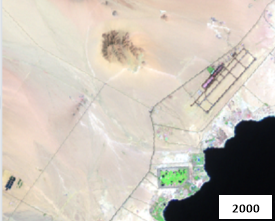
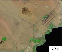
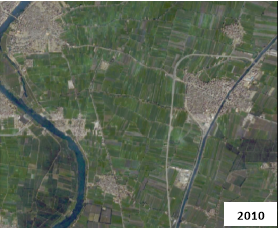
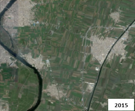
Figure (3.4) illustrates the second dataset of a village belongs to EL Mahalla al-Kubra city in Egypt. It consists of two images acquired in 2010 and 2015. It is taken by El-Shayal Smart web online Software that could acquire Satellite images from Google Earth. The image area lies between Lat. 30 57 46.9032 N, Lon. 31 14 35.4776E and Lat. 30 54 47.00 N, Lon. 31 18 19.98. Table (3.2) summarizes the characteristic of this dataset.
|
|
|
|
(a) |
(b) |
|
Fig ( 3.4 ) Dataset of EL mahalla al-kubra city- Egypt ( Google Earth) (a) image acquired at 2010 and (b) image acquired at 2015. |
|
|
No |
Spatial resolution |
Radiometric resolution |
Number of bands |
Acquisition date |
Size [pixels] |
Area [km2] |
|
|
Width |
Height |
||||||
|
1 |
6 m |
8 bits |
3 |
2010 |
1056 |
1007 |
38.2821 |
|
2 |
6 m |
8 bits |
3 |
2015 |
1056 |
1007 |
38.2821 |
1.4 Image Pre-processing for Change Detection
Before change detection process, it is usually necessary to carry out the radiometric correction and image registration for the dataset used [64]. In sections 3.4.1and 3.4.2, the concept of radiometric and image registration are described. The execution of preprocessing on the dataset used is given in section 3.7.2.
1.4.1 Radiometric correction
Radiometric conditions are influenced by many factors such as different imaging seasons or dates, different solar altitudes, different view angles, different meteorologic conditions and different cover areas of cloud, rain or snow etc. It may affect the accuracy of most change detection techniques. Radiometric correction is performed to remove or reduce the inconsistency between the values surveyed by sensors and the spectral reflectivity and spectral radiation brightness of the objects, which encompasses absolute radiometric correction and relative radiometric correction [26].
- Absolute radiometric correction
It mainly rectifies the radiation distortion that is irrelevant to the radiation features of the object surface and is caused by the state of sensors, solar illumination, and dispersion and absorption of atmospheric etc. The typical methods mainly consist of adjusting the radiation value to the standard value with the transmission code of atmospheric radiation, adjusting the radiation value to the standard value with spectral curves in the lab, adjusting the radiation value to the standard value with dark object and transmission code of radiation, rectifying the scene by removing the dark objects and so on. Due to the fact that it is expensive and impractical to survey the atmospheric parameter and ground objects of the current data, and almost impossible to survey that of the historical data, it is difficult to implement absolute radiometric correction in most situations in reality.
- Relative radiometric correction
In a relative radiometric correction, an image is regarded as a reference image. Then adjust the radiation features of another image to make it match with the former one. Main methods consist of correction by histogram regularization and correction with fixed object. This kind of correction can remove or reduce the effects of atmosphere, sensor, and other noises. In addition, it has a simple algorithm. So it has been widely used. The radiation algorithms that are most frequently used at present in the preprocessing of change detection mainly consists of image regression method, pseudo-invariant features, dark set and bright set normalization, no-change set radiometric normalization, histogram matching, second simulation of the satellite signal in the solar spectrum and so on. It should be pointed that radiometric correction isn’t necessary for all change detection methods. Although some scholars hold that radiometric corrections are necessary for multi-sensor land cover change analysis Leonardo studies at 2006 have shown that if the obtained spectral signal comes from the images to be classified, it is unnecessary to conduct atmospheric correction before the change detection of post-classification comparison. For those change detection algorithms based on feature, object comparison, radiometric correction is often unnecessary [64].
1.4.2 Image registration
Precise registration to the multi-temporal imageries is essential for numerous change detection techniques. The importance of precise spatial registration of multi-temporal imagery is understandable because generally spurious results of change detection will be formed if there is misregistration. If great registration accuracy isn’t available, a great deal of false change area in the scene will be caused by image displacement. It is commonly approved that the geometrical registration accuracy of the sub-pixel level is recognized. It can be seen that the geometrical registration accuracy of the sub-pixel level is necessary to change detection. However, it is doubtful whether this result is suitable for all registration data sources and all detected objects and if suitable how much it is. Another problem is whether this result has no influence on all change detection techniques and applications and if there is any influence how much it is. These Problems are worth to be studied further. On the other hand, it is difficult to implement high accuracy registration between multi-temporal especially multi-sensor remote sensing images due to many factors, such as imaging models, imaging angles and conditions, curvature and rotation of the earth and so on. Especially in the mountainous region and urban area, general image registration methods are ineffective and orthorectification is needed. Although geometrical registration of high accuracy is necessary to techniques used for low, medium and high resolution (like image differencing techniques and post-classification), it is unnecessary for all change detection t. For the feature-based change detection methods like object-based change detection method, the so-called buffer detection procedure can be employed to associate the extracted objects or features and in this manner, the harsh prerequisite of perfect registration can be escaped [65]. However, these methods neglect the key problem of the distinction between radiometric and semantic changes. So, it does not address the problem of change detection from a general perspective. It just focuses on specific applications relevant to the end user [1].
1.5 Accuracy Assessment used for Change Detection Process evaluation
The accuracy of change detection depends on many factors, including precise geometric registration and calibration or normalization, availability and quality of ground reference data, the complexity of landscape and environment, methods or algorithms used, the analyst’s skills and experience, and time and cost restrictions. Authors in [66] summarized the main errors in change detection including errors in data (e.g. image resolution, accuracy of location and image quality), errors caused by pre-processing (the accuracy of geometric correction and radiometric correction), errors caused by change detection methods and processes (e.g. classification and data extraction error), errors in field survey (e.g. accuracy of ground reference) and errors caused by post-processing.
Accuracy assessment techniques in change detection originate from those of remote sensing images classification. It is natural to extend the accuracy assessment techniques for processing single time image to that of bi-temporal or multi-temporal images. Among various assessment techniques, the most efficient and widely-used is the error matrix [26]. It describes the comparison or cross-tabulation of the classified land cover to the actual land cover revealed by the sample sites results in an error matrix as demonstrated in the table (3.3). It can be called a confusion matrix, contingency table [67], evaluation matrix [68] or misclassification matrix [69]. Different measures and statistics can be derived from the values in an error matrix. These measures are used to evaluate the change detection process. These measures are overall accuracy, procedures accuracy and user accuracy [70].
- Overall accuracy of the change map
It presents the ratio of the total number of correctly classified pixels to the total number of pixels in the matrix. This figure is normally expressed as a percentage. It can be expressed as follows:
The overall accuracy = 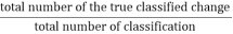 (3.1)
(3.1)
- User’s accuracy (column accuracy)
It is a measure of the reliability of change map generated from a CD process. It is a statistic that can tell the user of the map what percentage of a class corresponds to the ground-truthed class. It is calculated by dividing the number of correct pixels for a class by the total pixels assigned to that class.
The user accuracy = 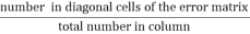 (3.2)
(3.2)
- Producer’s accuracy (raw accuracy)
It is a measure of the accuracy of a particular classification scheme. It shows what percentage of a particular ground class was correctly classified. It is calculated by dividing the number of correct pixels for a class by the actual number of ground truth pixels for that class.
The procedure accuracy =  (3.3)
(3.3)
|
Classified land cover |
|||
|
Actual land cover |
Class1 = change |
Class2 = no change |
|
|
Class1 = change |
Correct |
False |
|
|
Class2 = no change |
False |
Correct |
|
1.6 Concepts of the selected change detection techniques
Seven LULC change detection techniques are selected to be implemented on our dataset. These techniques are post-classification, direct multi-date classification (DMDC), image differencing (ID), image rationing (IR), image symmetric relative difference (ISRD), change vector analysis (CVA), and principal component differencing (PCD).
- Image differencing
Itis based on the subtraction of two spatially registered imageries, pixel by pixel, as follows:
ID =Xi (t2) – Xi (t1) (3.4)
Where:
- X represents the multispectral images with I (number of bands) acquired at two different times t1and t2.
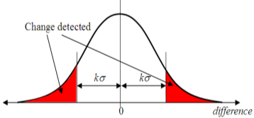
The pixels of changed area are predictable to be scattered in the two ends of the histogram of the resulting image (change map), and the no changed area is grouped around zero as shown in figure (3.5). This simple manner easily infers the resulting image; conversely, it is vital to properly describe the thresholds to perceive the change from non-change regions [71].
|
|
- Image Rationing
It is similar to image differencing method. The only difference between them is the replacement of the differencing images by rationed images [71].
IR =Xi (t2) / Xi (t1) (3.5)
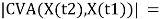
- Image Symmetric Relative Difference
it is based on the useof symmetric relative difference formula to measure change [72], as follows:
ISRD = 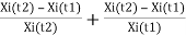 (3.6)
(3.6)
Separating the change by the pixel’s value at time 1 and time 2 permits the derivation of a change map that measures the proportion change in the pixel, nonetheless of which image is selected to be the first image. For instance, a pixel that had a value of 20 at time 1 and a value of 80 at time 2 would have an absolute change of 60, and a proportion change value in the change map of 375%:
[(80 – 20) / 20 + (80-20)/80] * 100 = 375%
An additional pixel with a value of 140 at time 1 and 200 at time 2 would also have an absolute change of 60, but its proportion change would only be 72.86%:
[(200 – 140) / 140 + (200-140)/200] * 100 = 72.86%
In general, it can be supposed that the proportion change of a pixel’s brightness value is more revealing of real change in the image than purely the absolute change [73].
- Change Vector Analysis
It generates two outputs: a change vector image and a magnitude image. The spectral change vector (SCV) explains the direction and magnitude of change from the first to the second date. The overall change extent per pixel is considered by defining the Euclidean distance between end points over dimensional change space, as follows:
 (3.7)
(3.7)
A decision on change is made based on whether the change magnitude exceeds a specific threshold. The geometric concept of CVA is applicable to any number of spectral bands [41].
- Principal Component Differencing
It is often accepted as effective transforms to derive information and compress dimensions. Most of the information is focused on the first two components. Particularly, the first component has the most information. The difference between the first principle component of two dates has the potential to advance the change detection outcomes, i.e.
PCD= PC1 (X(t2)) – PC1 (X(t1)) (3.8)
The change detection is implemented based on threshold [28].
- Direct multi-date classification
It combines the two images (X (t2) and X (t1)) into a single image on which a classiï¬cation is performed. The areas of changes are expected to present different statistics (i. e., distinct classes) compared to the areas with no changes [74].
- Post-classification
It is based on the classification of the two images (X (t2) and X(t1)) separately and then compared. Ideally, similar thematic classes are produced for each classiï¬cation. Changes between the two dates can be visualized using a change matrix indicating, for both dates, the number of pixels in each class. This matrix allows us to interpret what changes occurred for a speciï¬c class. The main advantage of this method is the minimal impacts of radiometric and geometric differences between multi-date images. However, the accuracy of the ï¬nal result is the product of accuracies of the two independent classiï¬cations (e.g., 64% ï¬nal accuracy for two 80% independent classiï¬cation accuracies) [74].
1.7 Experimental work
This section describes the environment and the implementation procedures of seven selected change detection techniques on the first dataset of Sham el-Sheikh city.
1.7.1 Experiment setup
Applying methods described in section 3.5 requires a suitable setup (environment). The setup requirements are summarized in software and hardware. A laptop machine with processor Intel(R) core (TM)i7-4500U CPU @1.80 GH 2.40 GH and RAM 8 GB is used as hardware environment. ERDASD IMAGINE 2014 is selected to be the software environment. It has the Model maker toolbox which is used as a programming language. It is chosen for its ability to combine matrix datasets and multi-dimensional arrays that are used to represent multi-dimensional images, and also for its ability to visualize and interrogate results in an interactive manner. Moreover, it allows providing the integration of the necessary datasets and algorithmic customizations for the development of the described method.
1.7.2 Pre-processing
Dataset of EL mahalla al-kubra described in section 3.3 had already registered before. Radiometric correction is carried out to minimize the false change detection by applying histogram matching between the two images. So, the pixel of the no changed areas in one date should take the same or close gray level values of the corresponding pixels in the other date as shown in figure (3.6) [75].
|
|
|
|
(a) |
(b) |
|
Fig (3.6 ) Dataset of Sharm el-Sheikh city after applying histogram matching on the image acquired at 2000 to match the image acquired at 2010. |
|

1.7.3 Implementation of the change detection techniques
The selected techniques are implemented by the model maker in the ERDAS IMAGINE 2014 software for a dataset of Sharm el-Sheikhto provide an overview and assessment of LULC change detection techniques. 250 random variables are used to generate an error matrix to calculate the overall accuracy according to equation (3.1). The reference points are driven visually by comparing the two images. Table (3.4) summarizes the implementation of the selected methods.
1.7.4 Results analysis
The results of applying the selected change detection techniques on the first dataset of Sham el-Sheikh city are introduced in the following:
- Image differencing
The change map generated using the image differencing method described in section 3.6 is shown in figure (3.7). The change map has two colors. The white color represents the changed area while the black color represents the no changed area. The change error matrix is generated using 250 random variables as demonstrated in the table (3.5). The reference information is taken visually by comparing the dataset. It is used to calculate the overall accuracy, user accuracy, and the procedures accuracy. The overall accuracy of the change map is 92.4%.
 of the two images.
Cite This Work
To export a reference to this article please select a referencing stye below:
Related Services
View all


DMCA / Removal Request
If you are the original writer of this essay and no longer wish to have your work published on UKEssays.com then please click the following link to email our support team:
Request essay removal