Buoyany Driven Flows in a Thermocline Cylinder with Sensible Heating

Buoyany Driven Flows in a Thermocline Cylinder with Sensible Heating

1.0 Introduction

Buoyancy driven flows, especially within enclosures, has been of great interest over the last 10 years. Buoyancy-driven natural convection in a heated cavity with differentially heated walls, maintained at a constant temperature, is a model for many industrial applications. One of the complexities of a flow within a cavity is the characteristic interplay of both the viscous and buoyancy forces of the fluid. Therefore, many experiments and numerical simulations have been reportedly conducted, in order to gain a better understanding of the flow and its properties. Rayleigh number, a dimensionless fluid property, dictates the buoyancy-driven flow within a cavity, which arises due to differences in gradients of the fluid. This is a model problem for many industrial applications e.g. heat recovery systems, energy-efficient design of buildings and rooms, gas-filled cavities around nuclear reactor cores, methods of cooling electronic devices, double glazed windows and solar energy instruments (i.e. thermal energy storage systems [thermocline tanks]). This research paper presents a numerical analysis of a thermocline tank, modelled as a square 2D cavity with differentially heated vertical walls. A commercial CFD package will be used to obtain solutions for the heat transfer of the two-dimensional natural convection flow model and express it in terms of global and local Nusselt numbers.

2.0 Literature review

The reliance upon fossil fuels for power generation coupled with an inadequate energy storage system has led to having the environmental concerns we currently observe. Being able to capture and store Carbon Dioxide has been extremely useful however, recently there has been an advancement in the energy sector. The storage of thermal energy as sensible heat in a thermocline cylinder has provided a platform for concentrated solar power (CSP) plants to generate electricity throughout the night without the use of fossil fuels.

With a development and utilisation of renewable energy sources in the energy sector, solar power has become increasingly popular as an alternative source of energy which can provide a considerable amount of power if utilised and optimised appropriately. It is estimated that the sun can provide solar energy for another 4 billion years, making this source of energy sustainable and renewable in the long-term (Davison, 2018). Thermal energy storage has a growing role in global deployment of power generation from solar power, due to their inherent intermittent nature.

2.1 Concentrated Solar Power (CSP)

Concentrated solar power (CSP) plants are anticipated to increase their presence in electricity markets, specifically because of their ability to integrate cost-effective thermal energy storage (TES) and create high efficiencies with notable scale up potential. When applied to concentrated solar power plants, thermal energy storage may allow for electricity generation at periods of limited sunlight i.e. nocturnal periods, which can correct the disparity between supply and demand. Traditionally in CSP plants, a tank storage system is implemented, where a heat transfer fluid acts as the primary heat storage medium in either one or two tanks (Alva, Lin and Fang, 2018).

The two-tank system can be configured as an indirect or direct system, where the biggest difference between them both is the heat transfer fluid (HTF) used in both the TES and solar field. For an indirect system, the working HTF within the TES is different to that of the HTF being pumped through the solar field. Due to this difference in the fluids, there is a requirement for an intermediate heat exchanger to facilitate heat transfer between both HTF. So, throughout daylight operations, the solar field HTF transports the gathered solar thermal energy to a power block, where there is a steam generating heat exchanger (i.e. boiler) and the surplus thermal energy is transferred to the TES HTF via the intermediate heat exchanger. The direct system works by using the same HTF for both the solar field and TES, therefore it does not require an intermediate heat exchanger. In the two-tank system, hot (heated) HTF is stored in one tank and cold HTF is stored in the other, so there is a temperature difference between them both. (Fasquelle et al., 2018)

2.2 Alternative storage options

The other storage method which is becoming increasingly popular in CSP plants is the use of a one tank system, called a thermocline tank. This storage method operates based on having fluid at dissimilar temperatures in the same tank. Due to temperature differences in the fluid, there is differences in the density between them both. Therefore, the higher temperature (less dense) fluid rises to the top of the tank and the colder, denser fluid falls to the bottom of the tank. There is an intermediate layer formed between the hot and cold fluid, which is called a thermocline, hence the name ‘thermocline’ tank.  This method of storage has many benefits, the obvious one being the need for just one tank rather than two, which will reduce costs by up to 35% in comparison to a two-tank storage configuration. (Tesfay and Venkatesan 2013).

All possible configurations for single tank and two-tank thermal energy storage systems can be seen below in figure 1.

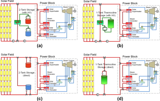
Figure 1: CSP plant configurations; (a) Indirect two-tank set up, (b) Single tank thermocline storage with heat exchanger, (c) Direct storage two-tank set up, (d) Single tank thermocline storage (direct) [Biencinto, M. et al. (2014)].

There have been different heat transfer fluids used in the past but the most common one used for recent studies is molten salt. This is because of some advantages which molten salts possess, they can raise the solar field output temperature to approximately 450-500°C, in so doing, this can increase the Rankine cycle efficiency of the power block steam turbine to ~ 40%. In comparison, the current high-temperature oil cycle efficiency is around 37.6% with an output temperature of 393°C. Kearney, D. et al. (2003).

2.3 Heat Transfer Mechanism

Heat transfer can be of three modes, conduction, convection and radiation. The heat transfer mechanism relies on temperature differences between systems as the driving force. Heat energy will move from a region of higher temperature to a region of lower temperature until there is equilibrium of the temperatures in the respective systems.

Conduction

Heat conduction can occur in solids, liquids and gases. The heat energy is transferred from high-energy particles to low-energy particles within the system as the particles interact with each other. These interactions differ dependent upon the fluid state interactions. For example, in solid state systems conduction occurs as the heat transfer is carried out by the vibration of molecules and the energy transport by free electrons. However, in liquids and gasses, the heat conduction occurs due to the collisions and diffusion of the molecules by their random motions.

Heat conduction is affected by two factors: the thickness and the density of the medium. So, at constant temperature conditions, the thickness of the medium will affect the heat energy that is transferred i.e. a thicker medium would allow less heat transfer and vice versa. Therefore, the thermal conductivity of gas is lower than liquids as the molecules of liquids are more closely spaced than gases. Based on these facts, we can conclude that the amount of heat transfer via conduction is proportional to the temperature differences across the medium but is inversely proportional to the thickness of the medium, this is equation is known as Fourier’s law of heat conduction;

${\mathrm{Q}}_{\mathrm{conduction}}=\mathrm{ }–\mathrm{kA}\frac{\mathrm{dT}}{\mathrm{dx}}$

Where;

A= Surface area, k= Thermal conductivity of material/substance, $\frac{\mathrm{dT}}{\mathrm{dx}}$

= Temperature gradient across medium

Convection

The heat convection mechanism occurs across fluid mediums and the integral feature for the heat transfer to occur is the motion of the fluid i.e. bulk movement of fluid particles. This mode of heat transfer can only take place across a temperature gradient and the equation that describes this is known as Newton’s law of cooling, which is;

${\mathrm{Q}}_{\mathrm{convection}}=\mathrm{hA}({\mathrm{T}}_{\mathrm{f}}–\mathrm{T})$

Where;

h= Convective heat transfer coefficient, A= Surface area, ${\mathrm{T}}_{\mathrm{f}}$

= Temperature at the surface, T= temperature of surrounding fluid

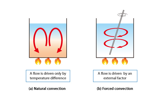
Convection can be split into two groups, forced convection and natural convection. As the name suggests, in forced convection the fluid motion is driven by an external force, whereas in natural convection, the fluid motion is driven by natural effects, such as buoyancy driven forces.

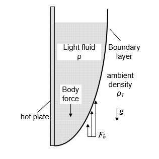
Buoyancy driven forces are a phenomenon whereby a lighter fluid gravitates upwards due to a net vertical force in a gravitational field. When heat energy is transferred from a solid substance to adjacent fluid substance via convection, the fluid will warm up and become relatively light. This light fluid will experience weight loss as the result of reduced gravity and gravitate upwards, whilst a cooler, more dense fluid will move downwards; this is then known as the buoyancy driven force.

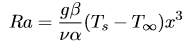
Fluid properties such as the Nusselt number (Nu), is the parameter which expresses the ratio of convective to conductive heat transfer ratio, which is the single most important parameter when looking at heat transfer configurations. Another important fluid property is the Rayleigh number (Ra), which is associated with buoyancy driven flows within fluids when natural convection is occurring. When a critical Ra value specified for a fluid is surpassed, the main mode of heat transfer occurs through convection.

Equation 1- Rayleigh number- Taken from [Iacovides, H. (2018).]

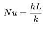
Equation 2- Nusselt number- Taken from Iacovides, H. (2018).

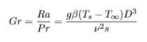
Other important dimensionless parameters are; the Reynolds number (equation 3), the Prandtl number (equation 4) and the Grashof number (equation 5). They represent the ratio of inertial force over viscous force (eq 3), the ratio of viscous diffusion over thermal diffusion (eq 4) and the ratio of buoyancy force over viscous force (eq 5). All five of these dimensionless parameters mentioned, play a crucial role in governing the physics of the flow.

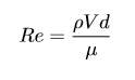
Equation 3- Reynolds number- Taken from Iacovides, H. (2018).

Equation 4- Prandtl number- Taken from Iacovides, H. (2018).

Equation 5- Grashof number- Taken from Iacovides, H. (2018).

2.4 Modelling & Simulation

Numerical simulation techniques, such as computational fluid dynamics (CFD), are widely used in recent times, to analyse the heat transfer problems in different application. The governing equations for CFD are the Navier-Stokes equations, which relate a fluids temperature, pressure and density of a moving fluid. The fluid flow domain is split up into subdomains/cells which as a collective are called a mesh/grid. The momentum and energy equations can be discretized using a numerical method, such as finite differencing, finite volume method etc. Employing a turbulence model, which describes the physical behaviour of the flow, will allow for the Navier-Stokes equations to model the turbulent flow. The fluid properties stated above can be inputted and other boundary conditions applied to solve complex heat transfer problems. This is an alternative to experimental procedures but data from both are always compared with each other.

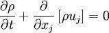
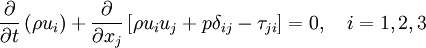
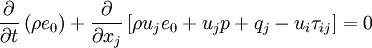
The Navier-Stokes equations {(6.0) Continuity, (6.1) Momentum, (6.2) Energy} are written below;

2.5 Discretization schemes

Fluid flows can be described by partial differential equations, which cannot be solved analytically due to complexities in the mathematics required, except in special cases. To obtain an approximate solution numerically, we must use a discretization method which approximates the differential equations by a system of algebraic equations, which can then be solved on a computer. Two of the main discretization methods are mentioned below;

Finite difference method- FDM

This is a numerical method for solving differential equations by way of approximating them and then replacing the derivatives in the equation using differential quotients. There are 3 forms which are commonly seen for FDM, which are; i) Forward differencing, ii) Backward differencing, iii) Central differencing. Taylor series expansion is used to obtain approximations to the first and second derivatives of the variables with respect to the coordinates. (Ahmadian, 2016)

$u\left(x\right)=\mathrm{ }\sum _{n=0}^{\mathrm{\infty }}\frac{(x–x_i{)}^n}{n!}(\frac{{\partial }^{n}u}{\partial x^n}{)}_i\mathrm{ }$

 Taylor series expansion    Eq 7.0

$(\frac{{\partial }^{n}u}{\partial x^n}{)}_i\mathrm{ }\approx \frac{u_{i+1}–u_i}{∆x}$

  Forward differencing

$(\frac{{\partial }^{n}u}{\partial x^n}{)}_i\mathrm{ }\approx \frac{u_i–u_{i–1}}{∆x}\mathrm{ }$

  Backward differencing

$(\frac{{\partial }^{n}u}{\partial x^n}{)}_i\mathrm{ }\approx \frac{u_{i+1}–u_{i–1}}{2∆x}$

    Central differencing

Finite volume method- FVM

This is a method used for finding a solution to partial differential equations (Navier-Stokes equations) in the form of a system of linear algebraic equations. It was named as such due to the small control volumes that surround the nodes on the mesh i.e. ‘finite volumes’. At each of these control volumes (CVs), the conservation equations are applied and the node which is located at the centre of each CV is where the variable values (pressure, velocity etc.) will be calculated and through interpolation, these values can be expressed at the CV surface in terms of the nodal values. (Ahmadian, 2016)

3.0 Navier-Stokes equations

As mentioned previously, the N-S equations are what govern the physics of the fluid flow motion. However, obtaining analytical solutions for these equations for complex, turbulent flows is not achievable but is available for simple laminar flows. Most fluid flow motions we encounter in real life are of a turbulent nature and three dimensional; therefore we require a method to obtain the solutions for the N-S equations.

One method to solve the N-S equations is through Direct Numerical Simulation (DNS), whereby the N-S equations are solved directly for all scales of turbulent eddies. This method requires no modelling to be done via a turbulence model and thus is very computationally expensive and time extensive. Therefore, making this method unfeasible except for simple, low Re number flows with simple geometries.

3.1 Reynolds Averaged Navier-Stokes

The prominent method is to use Reynolds Averaged Navier-Stokes (RANS) equations, which are time-averaged equations for fluid flow motion alongside a turbulence model. This method decomposes the flow variables into mean and fluctuating parts and inserts them into the N-S equations. Through an averaging of the equations, an unknown term called the Reynolds stress tensor arises, which then will be modelled to solve the RANS equations. The decomposition of turbulence is as such;

$u_i\left(\overline{x},y\right)=\mathrm{ }{U}_i\left(\overline{x}\right)+u_i‘(\overline{x},\mathrm{ }t)$

     eq 8.0

Where the velocity at any time interval is $u_i$

, $U_i$

is the mean velocity component and $u_i^{‘}$

is the fluctuating component. Using the equation above, the N-S equations are averaged, either through time-averaging or ensemble averaging. Depending on nature of the flow simulation (steady-state or transient), one of these averaging processes will be used. For steady-state simulations, where there is a time independency, a time averaging process is applied. A transient simulation, a time dependent flow, would therefore use ensemble averaging.

The RANS equation written in index notation for an incompressible fluid (Newtonian) is shown below.

$\rho \frac{\partial u_i}{\partial t}+\rho {\overline{u}}_j\frac{\partial u_i}{\partial x_i}=\rho {\overline{f}}_i+\mathrm{ }\frac{\partial }{\partial x_j}[–\overline{p}{\delta }_{\mathit{ij}}+\mu \left(\frac{\partial {\overline{u}}_i}{\partial x_j}+\mathrm{ }\frac{\partial {\overline{u}}_j}{\partial x_i}\right)\mathbf{–}\mathbf{ }\overline{\mathit{\rho }{\mathit{u}}_{\mathit{i}}^{\mathbf{‘}}{\mathit{u}}_{\mathit{j}}^{\mathbf{‘}}}]$

As mentioned previously, after the averaging process, there arises an unknown term; the Reynolds stress tensor;

${\tau }_{\mathit{ij}}=\mathrm{ }–\overline{\mathit{\rho }{\mathit{u}}_{\mathit{i}}^{‘}{\mathit{u}}_{\mathit{j}}^{‘}}$

As mentioned before, the above equation can be modelled to solve the RANS equations. The components of the equation above, must be solved in order to close the system. The turbulence model chosen will be modelling the Reynolds stress tensor and generally should be widely applicable to a range of applications, with an acceptable accuracy and reasonably computationally inexpensive.

3.2 Boussinesq Hypothesis

The Boussinesq hypothesis is used to introduce ‘eddy viscosity’ which models the momentum transfer due to turbulent eddies. It is used to attain two-equation turbulence models (more information on two-equation models below). For incompressible flows, the Reynold stresses are modelled by the following equation;

$\mathrm{\rho }{\mathrm{\tau }}_{\mathrm{ij}}={\mathrm{\mu }}_{\mathrm{t}}\left[\frac{\partial U_i}{\partial x_j}+\frac{\partial U_j}{\partial x_i}\right]–\frac{2}{3}{\delta }_{\mathit{ij}}\mathit{\rho k}$

Where ${\mathrm{\mu }}_{\mathrm{t}}$

is the eddy viscosity, $k$

is the turbulent kinematic energy and $U_i$

is the mean velocity component. By using this hypothesis, the number of Reynold stresses (six) can be whittled down to two unknown variables, ${\mathrm{\mu }}_{\mathrm{t}}$

and $k$

, where $k$

is defined as;

$k=\frac{1}{2}\overline{u_i^{‘}{u}_j^{‘}}$

Scalar quantities such as density, mass etc. can also be modelled in a similar fashion. The turbulence transport of these quantities can be expressed as;

$–\mathrm{\rho }\overline{{\mathrm{u}}_{\mathrm{i}}^{‘}{\mathrm{\phi }}^{‘}}={\mathrm{\Gamma }}_{\mathrm{t}}\frac{\mathrm{\delta \Phi }}{\mathrm{\delta }{\mathrm{x}}_{\mathrm{i}}}$

Where ${\mathrm{\Gamma }}_{\mathrm{t}}$

is the eddy diffusivity. Since both modelling of momentum and scalar turbulence transport are very similar in nature, the values of ${\mathrm{\Gamma }}_{\mathrm{t}}\mathrm{ }{\mathrm{\mu }}_{\mathrm{t}}$

are very close. Most open source CFD solvers and all commercial CFD solvers implement the Boussinesq hypothesis in their software.

3.3 Turbulence models

There are different classifications of RANS turbulence models that exist, such as; Zero-equation models, One-equation models, Two-equation models and further, more advanced Stress-equation models.

Zero-equation models involve solving a system of PDEs (partial differential equations) for the mean field only; they do not require any other PDEs. However, as you move up the classification order, the number of additional transport equations used increases, as the names would suggest. One-equation models use an additional transport equation which is used to calculate the turbulence velocity scale (also cast as average turbulent kinetic energy (K)). Two-equation models add another transport equation with respect to one-equation models. This additional transport equation is used to calculate the turbulence length scale (also cast as dissipation rate (ε)). The stress-equation models have multiple transport equations, catering for the Reynolds stress tensor $\left({\tau }_{\mathit{ij}}\right)$

and one for the dissipation rate (ε).

A zero-equation model is also known as an algebraic model- they are highly empirical. An example of a zero-equation model is the mixing length hypothesis developed by Ludwig Prandtl in the early 20^th century. This hypothesis works well with simple flows but does not hold well with complex, highly turbulent flows. One of the most well-known one-equation models is the Spalart-Allmaras model, generally this classification of turbulence models is implemented in the aerospace industry, as it is a reasonably simple turbulence model and is relatively computationally inexpensive. The $k–\omega \mathit{ k}–\epsilon$

turbulence models are classified as two-equation models and are highly popular in industry due to certain characteristics they have. They are relatively accurate and economical and more importantly, they have been validated through industry and academia for several flow problems. Depending on the flow conditions (i.e. low Reynolds number flows, transitional flows etc.), both turbulence models can be modified in order to solve specific flow conditions. For more complex turbulence models (i.e. stress-equation models), such as the Reynolds stress transport models (RST), they are not used in industry that often compared with two-equation models. This is mainly due to them being computationally expensive and lacking proper validation through industry and academia. As computational power and capabilities increase exponentially, the interest in higher classification turbulence models is being renewed.

3.3.1 Prandtl’s mixing length hypothesis (MLH) Zero-equation model

The MLH model was developed by Prandtl in 1925 by assuming the Reynolds stresses that are produced via momentum transfer can be expressed by means of an ‘eddy viscosity’. The Boussinesq eddy viscosity model can be expressed in the general form;

$–\overline{u_i^{‘}{u}_j^{‘}}={\nu }_t\left(\frac{\partial U_i}{\partial x_j}+\frac{\partial U_j}{\partial x_i}\right)–\frac{2}{3}{\delta }_{\mathit{ij}}k$

Where k= $\frac{1}{2}\overline{u_m^{‘}{u}_m^{‘}}$

and ${\nu }_t$

is termed the eddy viscosity. When analysing a thin shear layer flow, the equation above can be given as;

$–\overline{u^{‘}{v}^{‘}}= {\nu }_t\frac{\partial U}{\partial y}$

The assumption Prandtl implemented was ${\nu }_t~u{\mathcal{l}}_m$

, where u is defined as the turbulent velocity and ${\mathcal{l}}_m$

is the mixing length, that is said to be the distance over which the transfer of momentum occurs in fluid elements. Additionally, he hypothesised that

$u~ {\mathcal{l}}_m\left|\frac{\partial U}{\partial y}\right|$

Therefore, the eddy viscosity can be written as;

${\nu }_t={\mathcal{l}}_m^2\left|\frac{\partial U}{\partial y}\right|$

  leading to $–\overline{u^{‘}{v}^{‘}}= {\mathcal{l}}_m^2\left|\frac{\partial U}{\partial y}\right|\mathrm{ }\frac{\partial U}{\partial y}$

As simple of a model this is, it has some drawbacks, the main one being that according to equation (…) the eddy viscosity would vanish and become zero when there is a zero-velocity gradient (i.e. $\frac{\partial U}{\partial y}=0$

). However, this is physically unrealistic and through experimentation, has shown to not be the case. Another issue with this model is the errors that are caused in heat transfer calculations due to the heat transfer being expressed as;

${\mathrm{{\rm Y}}}_t\approx {\nu }_t={\mathcal{l}}_m\left|\frac{\partial U}{\partial y}\right|$

So, when $\frac{\partial U}{\partial y}=0$

this would suggest that the heat transfer (diffusivity) would be equal to zero. This can cause significant errors when calculating heat transfer in a flow.

3.3.2 Spalart-Allmaras One-equation model

This model solves a modelled transport equation for the eddy viscosity and as mentioned previously, is a one-equation model. The main usage of this model is within the aerospace industry (wall bounded flows) and is particularly suited to be implemented in problems which have adverse pressure gradients in the boundary layer. Of late, this model has also been used in turbo-machinery applications. This model has its weaknesses when dealing with low Reynolds number flows. This model is used to solve a transport equation for a viscosity like variable $\tilde{\nu }$

defined as,

$\frac{\partial \tilde{\nu }}{\partial t}+{\mu }_j\frac{\tilde{\nu }}{\partial x_j}=C_{b1}\left[1–f_{t2}\right]\tilde{S}\tilde{\nu }+\frac{1}{\sigma }\left\{\nabla .\left[\left(\nu +\tilde{\nu }\right)\nabla \tilde{\nu }+C_{b2}{\left|\nabla \nu \right|}^2\right]\right\}–[C_{w1\mathit{fw}}–\frac{C_{b1}}{{\kappa }^2}{f}_{t2}](\frac{\tilde{\nu }}{d}{)}^2+f_{t1}∆U^2$

   eq

This equation characterizes the transport equation where $∆U^2$

represents the velocity difference at the tip of the field and the field point, d represents the distance from the closest surface. The other terms in the equation are listed below. 

Where the eddy viscosity is given as;

${\nu }_t=\tilde{\nu }{f}_{u1}$

,  $f_{u1}=\frac{{\chi }^3}{{\chi }^3+C_{\mu 1}^3}\mathit{ },\mathit{ \chi }=\frac{\tilde{\nu }}{\nu }$

And the other terms in equation (…) are;

$\tilde{S}\equiv S+\frac{\tilde{\nu }}{{\kappa }^2{d}^2}{f}_{u2}\mathit{ }{f}_{u2}=1–\frac{\chi }{1+\chi f_{u1}}$

$f_w=g[\frac{1+C_{w3}^6}{g^6+C_{w3}^6}{]}^{\frac{1}{6}}\mathit{ g}=r+C_{w2}\left(r^6–r\right)\mathit{ r}\equiv \frac{\tilde{\nu }}{\tilde{S}{\kappa }^2{d}^2}$

$f_{t1}=C_{t1}{g}_t\exp \left(–C_{t2}\frac{{\omega }_t^2}{∆U^2}\left[d^2+g_t^2{d}_t^2\right]\right)$

$f_{t2}=C_{t3}\exp \left(–C_{t4}{\chi }^2\right)$

$S=\sqrt{2{\mathrm{\Omega }}_{\mathit{ij}}{\mathrm{\Omega }}_{\mathit{ij}}}$

Where ${\mathrm{\Omega }}_{\mathit{ij}}$

is defined as the rotational tensor;

${\mathrm{\Omega }}_{\mathit{ij}}=\frac{1}{2}\left(\frac{\partial u_i}{\partial u_j}–\frac{\partial u_j}{\partial x_i}\right)$

In order to solve this equation, there are closure coefficients required for this specific model, the Spalart-Allmaras model, summarised in table 1 below.

Table 1: Closure coefficients for the Spalart-Allmaras model.

3.3.3 Standard $\mathit{k}\mathit{–}\mathit{ϵ}$

two equation model

Launder and Spalding [REF] proposed this model back in 1972 and since its inception, this model has become widely used and popular in academia and industry because it has been validated many times and also because one of the traits of the model is the relatively low computational costs attached to it. This model was created by applying the Boussinesq hypothesis to the Reynolds stress terms and through this they obtained two more transport equations which had to be solved in order to close the RANS equations. The two additional equations relate to two variables that are to be determined, the turbulent dissipation $\mathit{ϵ}$

and the turbulent kinetic energy $\mathit{k}$

.

RANS (EVM, RSM)

LES

4.0 Case studies

Natural convection in cavities has been studied for many years. Batchelor (1954) formulated the problem of natural convection in a rectangular cavity, analysing the heat transfer behaviour using different values of the Rayleigh number. Wilkes and Churchill (1966) studied natural convection in a rectangular enclosure with differentially heated side walls using a finite difference scheme.

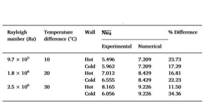
Srivastava et al. 2018 carried out both an experimental and numerical analysis on a differentially heated vertical closed cavity, to investigate the convective heat transfer which occurs within the cavity when certain boundary conditions are applied. Constant wall temperature differences were chosen to be (ΔT=10, 20 and 30°C) across the vertical side walls, whereas the horizontal walls were assumed to be adiabatic. The Rayleigh number variation was selected to be (Ra=9.7×10⁵, 1.8×10⁶ and 2.5×10⁶). A comparison between the experimental and simulated results was represented in the form of temperature contours, spatial distribution of the Nusselt number and spatially-averaged heat transfer rates as a function of Rayleigh number. The main findings from the analysis were that dominant corner flows were observed which could influence heat transfer rates. Consequently, the maximum heat transfer rates were seen near the bottom section of the hot wall and top section of the cold wall respectively. As the Rayleigh number increases, so does the average and maximum Nusselt numbers from both experimental and numerical datasets. Table one below summarises the results obtained from Srivastava et al. 2018.

Markatos and Pericleous (1984) were one of the first to take into consideration turbulence in their model for calculations. Through two-dimensional simulations, they varied the Rayleigh number (Ra) up to 10¹⁶ with a Prandtl number of (Pr=0.71) and produced graphs for the different values of Ra (Pr = 0.71). These values were plotted against Nusselt number to obtain a correlation between both variables and a good agreement was found through comparison of their simulation data and experimental data taken from [MacGregor and Emery, 1969]. Further results were shown in the form of isotherms, streamlines and velocity fields. The same numerical set up was used by Ozoe et al. [turbulence model (k- $\epsilon$

)] for Rayleigh numbers up to Ra = 10¹¹ and for an aspect ratio of A = 2. The results for the heat transfer were presented together with a parametric study of the k- $\mathit{ \epsilon }$

model constants and oscillations were found for the stream function at high Ra numbers but a general agreement with experimental results were found.

Henkes et al. (1991) carried out two-dimensional calculations of a square cavity which has vertical, differentially heated walls. The governing equations were solved using numerous mesh sizes by finite volume method. They used three different discretization schemes; the second-order central differencing, hybrid scheme and first-order upwind scheme. The central difference scheme was found to give the most accurate solutions for the heat transfer analysis. Both laminar and turbulent flow cases with Rayleigh numbers, ranging up to 10¹⁴ for air and 10¹⁵ for water were also performed. For the turbulence two-dimensional simulation, different versions of the k- $\mathit{ \epsilon }$

turbulence model were used. The two versions that were used were, the standard k- $\epsilon$

and low-Reynolds number k- $\epsilon$

models. Their results showed a good agreement between the numerical and experimental results even for high Ra (up to 10¹⁴), just as [Markatos and Pericleous, 1984]. The simulations were performed for air and water and results for the correlations between Nu and Ra were presented. From the results, it was clear that the low-Reynolds-number k- $\mathit{ \epsilon }$

model gave a better, more accurate result when compared with experimental data. They made a conscious effort to specify as many relevant parameters such as (geometry, k- $\mathit{ \epsilon }$

constants, grid discretization) so that results can be compared with other work by different researchers.

Jaballa et.al. (2017), carried out a numerical, two-dimensional analysis of natural convection heat transfer in a differentially heated square cavity. The Navier-Stokes and energy equations were solved using a finite volume method. The sidewalls were differentially heated, with the left wall being heated and the right wall was kept at a constant lower temperature. The Rayleigh number was varied from 10³ to 10⁸ whilst using a fluid with Prandtl number of 0.71 (air). One of the main findings was, at low Rayleigh numbers, the heat transfer was dominated by conduction but as the Rayleigh number was increased, the effects of convection became stronger. Results were shown through streamlines and isotherms and the average and local Nusselt numbers were obtained and compared with previous literature works.

Zaman et.al. (2013) conducted a two-dimensional, numerical simulation of natural convection flow in a rectangular enclosure for air with two discrete heaters, heating the bottom wall with an adiabatic section between them. Using an implicit finite difference method in conjunction with successive over relaxation (SOR) method to solve the governing, non-dimensional equations (Navier-Stokes and energy equation).  The Rayleigh number is varied from 10³ to 10⁷ and the corresponding heat transfer rates expressed in terms of the average and local Nusselt number is shown graphically. An observation was made that the heat transfer rate is practically zero close to the adiabatic section of the bottom wall. Also, a significant increase in the heat transfer rate was seen at the edges of the cavity across the bottom wall. Other numerical results such as temperature variations are shown in the form of isotherm and streamline.

De Vahl Davis’ (1983) numerical solution for natural convection in a square cavity is widely used as the benchmark data for comparison. The study is performed on a Boussinesq fluid (i.e. air), which has a Prandtl number 0.71 and for varying Rayleigh numbers of 10³ to 10⁶. The governing equations of motion and heat transfer are solved using a second-order central difference scheme with several mesh refinements. The vertical walls are differentially heated and maintained at T_h and T_c respectively. The horizontal walls are insulated and assumed adiabatic and the velocity components on the boundaries are assumed to be zero. For two-dimensional, incompressible flows within a cavity with constant fluid properties, a simplification of the Navier-Stokes equations can be done by using a stream function-vorticity formulation. This will produce a non-dimensional equation which can be solved using a finite difference method. The heat flux across the walls was calculated using a second order differencing approximation. Simpson’s rule was used to integrate the heat flux equation in order to obtain the average Nusselt number values. Richardson extrapolation was done to attain a higher order of accuracy of results, which were presented as the benchmark solutions. The results for the average Nusselt number throughout the cavity and the maximum and minimum Nusselt numbers across the boundaries in the vertical direction are clearly presented in a table format, with their respective locations along the wall. A clear trend was presented, which showed as the Rayleigh number increased, so does the Nusselt number which corresponds to a higher heat transfer rate along the vertical walls.

Le Quéré (1990) added more results for Ra = 10⁷ and Ra = 10⁸ (air) to the benchmark results from De Vahl Davis. Le Quéré used a different numerical scheme to solve the Navier Stokes and energy transport equations. The scheme which was used was a pseudo-spectral Chebyshev collocation method. An important outcome from the results was the significant size of the linear thermal stratification of the core and the detachment region at the horizontal adiabatic walls. As the Rayleigh number was increased, the flow eventually becomes unsteady.

Mention the gap in knowledge to be filled, i.e. how a certain shape may affect the buoyancy forces etc…

Conclusion

One tank thermal energy storage systems, such as thermocline tanks are becoming more prevalent amongst CSP power plants, used as a method to store thermal energy directly obtained from the sun. Integrating these tanks into a power generation system can enable CSP plants to produce electricity throughout nocturnal periods and fix the disproportionality between supply and demand of power generated through solar energy throughout the day. Thermocline regions are produced and maintained by the presence of density gradients within the fluid. The Rayleigh number is a dimensionless fluid property that is related to buoyancy-driven flows otherwise known as, natural convection. It is essential the tank retains as much thermal energy stored inside it as possible, to allow a higher working efficiency of the system. Therefore, heat transfer analysis is done on the heated cavity to determine the thermal efficiency of the thermocline tank, which is indicated by the heat transfer rate (i.e. how much thermal energy is being lost). The heat transfer rate is expressed in terms of the Nusselt number and this study will attempt to show how the Nusselt number varies with respect to the Rayleigh number by having a range of values for the Rayleigh number. Different geometry and boundary conditions set for the cavity may alter the heat transfer rate, such as having rectangular or triangular cavities. Or having the horizontal walls being differentially heated rather than the vertical walls or applying a constant heat flux rather than constant temperature to heated walls. Further research will attempt to address this gap in order to fully comprehend all aspects of this problem.

References

• Alva, G., Lin, Y. and Fang, G. (2018). “An overview of thermal energy storage systems”, Energy, 144, pp. 341-378. [Online]. available at: https://www.sciencedirect.com/science/article/pii/S036054421732056X (Accessed: 19 November 2018).
• Batchelor, G. (1954). “Heat transfer by free convection across a closed cavity between vertical boundaries at different temperatures”, Quarterly of Applied Mathematics, 12(3), pp. 209-233. (Accessed: 22 November 2018).
• Biencinto, M. et al. (2014). “Simulation and assessment of operation strategies for solar thermal power plants with a thermocline storage tank”, Solar Energy, 103, pp. 456-472. [Online]. available at: https://www.sciencedirect.com/science/article/pii/S0038092X1400125X (Accessed: 14 November 2018).
• Davison, A. (2018). Solar energy as Renewable and alternative energy, Solar technology & energy information, Altenergy.org. [Online]. available at: http://www.altenergy.org/renewables/solar.html (Accessed: 8 December 2018).
• De Vahl Davis, G. (1983). “Natural convection of air in a square cavity: A bench mark numerical solution”, International Journal for Numerical Methods in Fluids, 3(3), pp. 249-264. [Online]. available at: https://onlinelibrary.wiley.com/doi/abs/10.1002/fld.1650030305 (Accessed: 3 December 2018).
• Fasquelle, T. et al. (2018). “Numerical simulation of a 50 MWe parabolic trough power plant integrating a thermocline storage tank”, Energy Conversion and Management, 172, pp. 9-20. [Online]. available at: (Accessed: 16 November 2018).
• Henkes, R., Van Der Vlugt, F. and Hoogendoorn, C. (1991). “Natural-convection flow in a square cavity calculated with low-Reynolds-number turbulence models”, International Journal of Heat and Mass Transfer, 34(2), pp. 377-388. [Online]. available at: https://www.sciencedirect.com/science/article/pii/001793109190258G (Accessed: 27 November 2018).
• Hiroyuki, O. et al. (1985). “Numerical calculations of laminar and turbulent natural convection in water in rectangular channels heated and cooled isothermally on the opposing vertical walls”, International Journal of Heat and Mass Transfer, 28(1), pp. 125-138. [Online]. available at: https://www.sciencedirect.com/science/article/pii/0017931085900146 (Accessed: 26 November 2018).
• Iacovides, H. (2018). Forced convection.
• Jaballa, M., Hawisa, J. and Rakhiyes, M. (2018). “NUMERICAL INVESTIGATION OF BUOYANCY DRIVEN LAMINAR FLOW IN A DEFERENTIALLY HEATED CAVITY”, Engineering research (University of Tripoli, Libya), (23), pp. 63-76. [Online]. available at: http://www.jer.edu.ly/PDF/Vol-23-2017/JER-05-23.pdf (Accessed: 1 December 2018).
• Kearney, D. et al. (2003). “Assessment of a Molten Salt Heat Transfer Fluid in a Parabolic Trough Solar Field”, Journal of Solar Energy Engineering, 125(2), p. 170. [Online]. available at: https://www.researchgate.net/publication/303190155_Assessment_of_a_molten_salt_heat_transfer_fluid_in_a_parabolic_trough_solar_field (Accessed: 19 November 2018).
• Le Quéré, P. (1991). “Accurate solutions to the square thermally driven cavity at high Rayleigh number”, Computers & Fluids, 20(1), pp. 29-41. [Online]. available at: https://www.sciencedirect.com/science/article/pii/004579309190025D (Accessed: 3 December 2018).
• MacGregor, R. and Emery, A. (1969). “Free Convection Through Vertical Plane Layers—Moderate and High Prandtl Number Fluids”, Journal of Heat Transfer, 91(3), p. 391. [Online]. available at: http://heattransfer.asmedigitalcollection.asme.org/article.aspx?articleid=1434706 (Accessed: 26 November 2018).
• Markatos, N. and Pericleous, K. (1984). “Laminar and turbulent natural convection in an enclosed cavity”, International Journal of Heat and Mass Transfer, 27(5), pp. 755-772. [Online]. available at: https://www.sciencedirect.com/science/article/pii/0017931084901455 (Accessed: 26 November 2018).
• Srivastava, A., Singh, S. and Kishor, V. (2018). “Investigation of convective heat transfer phenomena in differentially-heated vertical closed cavity: Whole field experiments and numerical simulations”, Experimental Thermal and Fluid Science, 99, pp. 71-84. [Online]. available at: https://www.sciencedirect.com/science/article/pii/S0894177718308732 (Accessed: 25 November 2018).
• Tesfay, M. and Venkatesan, M. (2013). “Simulation of thermocline thermal energy storage system using C”, International Journal of Innovation and Applied Studies, 3(2), pp. 354-364. [Online]. available at: http://www.ijias.issr-journals.org/authid.php?id=311 (Accessed: 4 December 2018).
• Wilkes, J. and Churchill, S. (1966). “The finite-difference computation of natural convection in a rectangular enclosure”, AIChE Journal, 12(1), pp. 161-166. [Online]. available at: https://onlinelibrary.wiley.com/doi/10.1002/aic.690120129 (Accessed: 22 November 2018).
• Zaman, F., Turja, T. and Molla, M. (2013). “Buoyancy Driven Natural Convection Flow in an Enclosure with Two Discrete Heating from below”, Procedia Engineering, 56, pp. 104-111. [Online]. available at: https://www.sciencedirect.com/science/article/pii/S1877705813004499 (Accessed: 1 December 2018).
• Ahmadian, A. (2016). Numerical models for submerged breakwaters. Amsterdam: Butterworth-Heinemann is an imprint of Elsevier, pp.Chapter 6- 93-108.