Empirical Tests On Capital Asset Pricing Model
| ✓ Paper Type: Free Assignment | ✓ Study Level: University / Undergraduate |
| ✓ Wordcount: 4396 words | ✓ Published: 22 May 2020 |
Abstract
The focal point of study of this assignment is the empirical testing of capital asset pricing model on London Stock Exchange. To test the CAPM, a collection of shares that belong to thirty UK companies for a fifteen year span beginning Jan 2004 and closing Dec 2018 have been taken into consideration in company with the returns from UK FTSE share price index and a 30 day Treasury bill from UK. We then calculate the first pass regression and the second pass regression by using data analysis tool in excel. Three hypothesis tests are conducted covering the null and alternate hypothesis in each of these tests. The validity of CAPM is also determined along with these three tests. Coefficients acquired from second pass data are in agreement with CAPM or not constitutes the first test. Test two determines if high risk and high returns are positively correlated. Test three ascertains if a linear relation exist between returns and betas.
Introduction
Capital Asset Pricing Model is an ideology which was introduced by William Sharpe and John Lintner and is still widely used in pricing the assets. It is a theory that helps in determining the cost of company’s funds and to judge if the portfolios are performing well or not. It is a powerful tool to assess the correlation of risks with return (Fama & French, 2004). To understand this model we first have to consider a model that has zero volatility. Zero volatility means zero risk. Returns do not fluctuate with the market in case of zero risk which only means that returns is risk free having a zero beta. A second situation is the one in which we consider an asset whose returns are in close adherence to the market returns. In this situation asset returns are equal to the market returns E(rA) = E(rM). A third situation is the one in which we consider a greater volatility in the asset returns compared to the market. Such asset earns higher returns compared to the market by the way of compensation which the investor gets for holding such additional risk. This relationship between returns on the asset and its correlation to the market risk can be derived through a mathematical equation as mentioned below
E(rA) = rf + βA (E(rm) – rf)
The equation represents the capital asset pricing model where (Womack & Zhang, 2003)
rf represents the risk free rate. US treasury bills are the safest and risk free as they are an investment in the government securities. They could not be considered as wholly risk free as the inflation factor makes its returns uncertain but in comparison to the other instruments they represent risk free rate in a much better way. Treasury bills having a short term maturity within 5 years are considered having no market risk with low inflation risk over different period of investments (Chen, 2013)
(E(rm) – rf) represents the return in excess of risk free rate of return
βA = An asset contains both systematic and unsystematic risk. The volatility in the returns of an asset with respect to that of the market is denoted by systematic risk. This volatility is measured by beta which takes into consideration the risk that each security possesses in the overall portfolio. The mathematical formula to derive beta is
Cov(rA, rM) / σ²M
rA represents the asset returns
rM represents the market returns
σ²M represents the volatility of the market return
Cov(rA, rM) represents the covariance between asset return and market return
To calculate the portfolio beta, each security’s beta is averaged, weighted by the market cap of individual security.
Thus the capital asset pricing model denotes that the investors are rewarded for taking extra risk which is represented by asset beta in addition to the risk free rate. Relationship of risk with return can be shown graphically through a diagram called securities market line (Womack & Zhang, 2003).
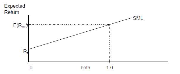
Figure 1.1
Markowitz Model is the base of capital asst pricing model. As per Markowitz’s model, investors dislike risk and they are concerned only about maximizing their returns, for a given level of risk or minimizing risk, for a given level of returns (Fama & French, 2004). This means that they do not consider other factors like skewness and kurtosis of distribution. Such portfolios are mean variance efficient (Chen, 2013). Markowitz model gives a mathematical statement on weight of the assets which is converted by the capital asset pricing model into a prediction that denotes relation between risk and return that can be tested by identifying an efficient portfolio (Fama & French, 2004)
Research Question
The objective of this assignment is to examine the CAPM’s validity on London Stock Exchange
Research Methodology
To examine Capital Asset Pricing Model is a two step process. Time – series regression or the first pass regression is the first step in two step process followed by cross sectional regression which is the second step. Dependent variable is security return or portfolio return and the return on market is an independent variable in the first step. The return on security is then regressed on market return so as to produce the coefficient of slope in the first pass regression. Coefficient of slope is the beta of the stock. The following equation of capital asset pricing model is used to regress the two variables: Rit = αi + βi Rmt + εit where
i is any company’s stock
t represents time period
Rit represents stock/portfolio returns at time t
Alpha (α) represents intercept of equation
Beta (β) represents slope coefficient of equation
Rmt is the market return at time t
Ε is the error term of regression equation
First pass regression helps us to produce Beta (β) of the security or portfolio which is then used in the cross sectional regression to calculate market premium. In cross sectional regression the variable which is dependent is excess return on security and the variable which is independent is the beta of the stock which we generate from the above equation. The excess return on security is regressed on stock Beta to generate risk premium (Bajpai & Sharma, 2015). The following equation is used to regress the two variables: Rj = γ0 + γ 1βj + ej where
Rj is the average return on stock/portfolio
γ0 is the intercept
βj is the sensitivity of stock derived from time series regression
ej is the error term (Theriou et al., 2005)
Literature Review
The first test for CAPM was conducted by John Linter. After Linter it was Douglas who conducted the test and his results for the tests were same as Linter. Two pass regression was used by Linter and a data of stocks with returns from 30 companies registered on NYSE from 1954 to 1963 was used by him. Linter used the two regression formulas = + ∗ + and = 0 + 1 1 + 2 2 ( ) + to find beta and second pass regression. CAPM is valid if the intercept which is Y0 is 0, slope of the assets beta which is Y1 is Rm –Rf and residual variance’s slope which is Y2 is 0. After the tests were conducted it was found that CAPM was not valid because intercept was much bigger when compared to any risk free rate, residual risk was not zero and SML slope Y1 and risk premium were not same.
Miller and Scholes too tested the CAPM following the same procedure and obtained the similar results like Linter. CAPM was not valid even in Miller and Scholes case. Both residual risk and intercept were not 0 and slope and risk premium were not same. In CAPM accurate numbers were set to meet the risk return relationship. These set up rates of return were in consent with CAPM. Their results were also same when compared with the results that were produced using real data therefore the CAPM that used the two step process was rejected. This showed that there were some statistical issues with two step process of CAPM because CAPM model was valid even if it was rejected when two step process was used. Error in measuring the beta is the reason why CAPM model was rejected. If the estimation of beta is unfair then the estimation of intercept will also be unfair (Jonsson & Asgeirsson, 2017). “By using said beta, estimated with a measurement error, in the second-pass regression will lead to a downward biased coefficient for the slope, y1, and an upward biased coefficient for the intercept, y0” (Jonsson & Asgeirsson, 2017, p. 11) These statistical problems made Miller and Scholes believe that two step process of CAPM was problematic.
According to Linter, Douglas, Miller and Scholes CAPM is invalid. It is not necessary that CAPM as a model is invalid. It can be simply due to the estimation of beta being unfair. In order that the estimation of beta is fair Black, Jensen & Scholes placed an emphasis on nature of security returns. They offered to group the securities rather than considering them individually so as to reduce the error in beta. Securities from 1926 – 1965 that were listed in NYSE were examined. Returns against the index were regressed for 60 months to estimate betas. In all there were 10 portfolios and in each of these portfolios the securities with highest to lowest betas were ranked. Such grouping of securities in portfolios based on their betas would still give them a measurement error. In order to avoid this, betas from the previous periods were used so that the portfolios for the following year were made. By doing so measurement error could be removed.
CAPM test was conducted by Sharpe and Cooper on stocks which were listed on NYSE from 1931 to 1967 with the aim to find out if higher betas had higher returns. Estimation of betas was carried out and then the ranking of shares was done on the basis of betas once a year and an equally weighted portfolio was formed by bifurcating the securities into 10 groups. Test conducted was successful as the results showed that higher betas had higher returns.
Fama and Macbeth tested the CAPM in a similar way like Black, Jensen and Scholes but he added one more parameter to it called beta square so as to find out if the correlation of risk with return is linear. Black, Jensen and Scholes used the beta of one particular period to predict the return of that same period but Fama and Macbeth use the beta of the previous period to predict the return of the following period. CAPM was tested using the equation = 0 + 1 + 2 2 + 3 2 + . The test concluded that a linear relationship existed between risk and return because y1 coefficient was not zero because of which slope was not negative and y2 and y3 coefficients were zero.
The first test on CAPM in the European stock market was conducted by Franco Modi in 1972. Before this the CAPM test was conducted only in the US markets because they were more efficient than European markets. The test was conducted on eight major markets in Europe and it was a replica of the test which was conducted before this in US market. The data for the test consisted of stocks from 235 countries in Europe from 1996 to 1971. The analysis of the data was done separately for each country. The results of the test showed that the market risk was an important element to be considered. Moreover risk and return showed a positive relation in seven countries out of eight.
David W. Mullins tested the CAPM and found out that the model was not perfect but was of the opinion that in order to determine the rate of return CAPM was a significant tool that could not be ignored by the investors.
The key findings of Pettengill, Sundaram & Mathur are that anticipated rather than realized returns are the basis for positive relationship between beta and returns as estimated by Sharpe Lintner Black model. Realized returns are considered as proxy for anticipated returns and the relationship of risk with returns is reversed when the excess market returns is negative.
Apart from the risk factor, Fama and Fench took size and book to market equity to study stocks. Their results are as follows: (Jonsson & Asgeirsson, 2017)
- “When we allow for variation in beta that is unrelated to size, there is not reliable relation between beta and average return.
- The opposite roles of market leverage and book leverage in average returns are captured well by book-to-market equity.
- The relation between E/P and average return seems to be absorbed by the combination of size and book-to-market equity” (Jonsson & Asgeirsson, 2017, p. 11)
Regression Output
Analysis is based on data collected from 1st Jan 2004 to 31 Dec 2018. The data consists of 30 company stocks that are registered on London Stock Exchange. With the help of this data we conduct our first pass regression and the results which we obtain from our first pass regression when excess stock returns and market returns are regressed, we get the beta of 30 companies which is demonstrated by the table below. We then regress the excess returns against the beta of 30 companies to get second pass regression. Second pass regression turns out to be -0.07456.
| Securities | Average Excess Return | Beta |
| RELX | 6.36% | 0.6970 |
| TED BAKER | 8.17% | 0.5915 |
| MARSTON’S | -4.38% | 1.2331 |
| BABCOCK INTERNATIONAL | 8.40% | 0.8715 |
| ITE GROUP | 1.54% | 1.5228 |
| COSTAIN GROUP | -1.58% | 0.5700 |
| MEGGITT | 4.76% | 1.3773 |
| 4IMPRINT GROUP | 17.59% | 1.1973 |
| CRH | 2.80% | 1.1108 |
| CONSORT MEDICAL | 3.35% | 0.5754 |
| INFORMA | 5.13% | 1.5128 |
| ASTRAZENECA | 3.42% | 0.5054 |
| ULTRA ELECTRONICS HDG. | 4.18% | 0.7531 |
| SAGE GROUP | 6.39% | 0.8910 |
| MENZIES (JOHN) | 2.25% | 1.3743 |
| ITV | -1.29% | 1.5256 |
| MORGAN ADVANCED MRA. | 2.93% | 1.8084 |
| BHP GROUP | 6.78% | 1.4745 |
| HILL & SMITH | 14.18% | 1.2154 |
| WOOD GROUP (JOHN) | 6.92% | 1.3596 |
| COMPASS GROUP | 7.93% | 0.7058 |
| BRITISH AMERICAN TOBACCO | 6.04% | 0.7034 |
| EASYJET | 7.00% | 0.6874 |
| REACH | -16.13% | 2.8017 |
| MCBRIDE | -0.38% | 0.7590 |
| MARSHALLS | 3.07% | 1.1385 |
| BROWN GROUP | -3.26% | 0.7441 |
| AVON RUBBER | 9.54% | 0.9746 |
| PETROPAVLOVSK | -22.45% | 1.7004 |
| BOOT (HENRY) | 6.41% | 0.9266 |
Table 1:1
Examining the capital asset pricing model
Three inferences are pillars which form the base on which the capital asset pricing model gets tested
- Expected returns on securities and beta’s are linearly related having no other variable that has marginal explanatory power
- The expected returns on market portfolio are more than the expected returns on the assets whereby the asset returns are uncorrelated with market returns. This indicates a positive risk premium.
- Returns on assets are equal to returns on risk free assets when the returns on assets have no correlation with the market returns. (Fama & French, 2004)
Heteroscedasticity and Autocorrelation
The econometric issue in the two pass test is that the ordinary least squares estimator becomes inefficient if the disturbance terms are heteroscedastic and correlated. Ordinary least squares estimator is inefficient when the degree of variance is higher for ordinary least squares estimator compared to the other estimators which in other words means that while testing the estimated coefficient the range of not rejecting the null hypothesis gets wider. Therefore the probability of accepting the null hypothesis increases even when the alternative hypothesis is true. Robust standard error is used to solve heteroscedasticity problem and general least square estimation is used to solve both heteroscedasticity and autocorrelation problem.
Measurement error in beta
The coefficient of slope called Beta is not observable in second pass data. It is derived either by using the formula Cov (Ri, Rm)/Var(Rm) or from the first pass regression of the two stage process. The estimated beta may be fair but it will surely contain a measurement error that will lead to ordinary least square estimators to be unfair and unstable. In individual assets measurement errors are higher compared to grouped portfolios therefore using grouped portfolios rather than individual assets is a solution so as to reduce measurement errors.
Time period and data frequency
Results for the estimation purposes would be more efficient if the data in the sample has more no of observations. So as to obtain more no of observations in the sample the time period for testing is to be extended in the time series regression or even the sampling frequency can be increased. If the time period for testing is not sufficient the estimation will not be fair and if it is sufficient a change in the relationship of regression can be observed. Moreover if the data is collected very frequently for example monthly then the efficiency of the estimation will decrease. Thus a monthly data over a period of five years is considered apt as beta tends to stabilize over a five year period (Chen, 2013)
Distinguishing first pass regression from second pass regression
“The tests of the CAPM provided by the time-series regression and the cross-section regression differ in terms of what is used as explanatory variable. In the time-series regression the explanatory variable is the excess market return, RMt – Rft, and we estimate βi. In the second-pass cross section regression the explanatory variable is bi, and we use the regression to construct a zero investment portfolio return, γ1t, whose expected value is the risk premium per unit of bi. Thus, the time series regression takes the market premium, RMt – Rft, as given and estimates βi, whereas the second-pass cross-section regression takes as given the cross-section of estimates of βi and uses them to produce a proxy for the market premium” (Fama, 2015, P.5)
The three factor model
A positive relationship exists between stock returns and beta as stated by capital asset pricing model. Cross sectional fluctuations in the stock returns are explained by only one component called beta. Research demonstrates that capital asset pricing model is partially capable to describe market anomalies like the reversals in the stock returns over a longer period or the short term fluctuations in the returns. Research also shows that a relation exists between stock returns and other factors like size of the firm, sales growth of previous years, earnings and cash flow per price, book to market equity. Capital asset pricing model is incapable of explaining the fluctuations in these returns in relation to the above mentioned factors which are popularly referred to as asset pricing anomalies. Three factor model of Fama and French is considered to be a better tool to describe cross sectional fluctuations in returns from stock rather than beta. Since beta is partially capable of explaining the cross sectional fluctuations, three factor model does so by adding two more factors that is firm’s size and book to market equity to the capital asset pricing model. Therefore the three factor model of Fama and French is considered to be an addition to capital asset pricing model. The mathematical form of three factor model is as follows:
E(Ri) – Rf = bi [E(Rm) – Rf] + siE(SMB)+hiE(HML)
E(Ri) – Rf represents the risk premium on portfolio i which can be elucidated by three factors (Xie & Qu, 2016) “(a) the market factor, measured by the difference between the market portfolio return RM and risk-free asset return Rf; (b) the size factor, SMB, measured by the difference between the return on a portfolio of small stocks and the return on a portfolio of large stocks; and (c) the value factor, HML, measured by the difference between the return on a portfolio of stocks with high book-to-market ratios and the return on a portfolio of stocks with low book-to-market ratios. E(*) denotes the expectation of premiums and the factor sensitivities. bi, si, and hi, are the slopes or sensitivities of expected risk premium of portfolio i to the market factor, size factor, and value factor in the regression.” (Xie & Qu, 2016, p. 1093-1094)
Roll Critique
Roll has criticized the test of asset pricing theory and demonstrates that a test on CAPM has never been conducted yet (Muthama et al., 2014). “He points out that tests performed by using any portfolio other than the true market portfolio are not tests of the CAPM but are tests of whether the proxy portfolio is efficient or not. Intuitively, the true market portfolio includes all the risky assets including human capital while the proxy just contains a subset of all assets” (Muthama et al., 2014, p. 611). If the correlation between proxy return and true return of the market is more than 0.70 then it is implied that the rejection of proxy CAPM also rejects true market portfolio CAPM as demonstrated by some studies. (Chen, 2013).
CAPM Assumptions
The CAPM assumptions are as follows
- No transaction costs
- No income tax
- Infinitely divisible assets
- Short selling is allowed
- No restriction on borrowing and lending at risk free interest rates
- Portfolios having efficient mean variance being held by individuals (Muthama et al., 2014)
- “A single period model
- All assets including human capital are marketable” (Muthama et al., 2014, p. 600)
- Expectation of investors with regards to the assets are homogeneous
- Stock prices cannot be influenced by buying and selling
- There should be a normal distribution of returns on securities.
- Investors should be reluctant to take risk and their behavior should be well reasoned, logical. They should have a utility maximizing attitude.
- Expected returns and their volatility should be the basis for investors decisions (Andor et al., 1999)
Hypothesis testing one
 The first test is performed with the objective to find out whether or not the coefficients acquired from second pass data are in agreement with CAPM. When we conduct hypothesis testing we create a hypothesis which is null and alternate. So in our case Y0 = 0 which is null & Y1 = (Rm-Rf) which is alternate. Y0 represents intercept and Y1 which is X variable 1 are the parameters of this test. The confidence interval for our test is 95%. The confidence interval of 95% with 29 observations gives us a range of +/-2.045. Thus if the Tstat value does not falls within this range of +/-2.045 the null hypothesis will be rejected. Through our calculations we get a T-stat value of 3.637. This value of 3.637446 is above the value of our range of +2.045. Therefore we reject null hypothesis. Validity of CAPM depends on intercept and slope. CAPM is valid if intercept is 0 and slope is equal to positive risk premium. In our case the intercept 0.114673 = 0. Therefore the CAPM is invalid. The average risk premium is -0.25. It is denoted by Y1. The risk premium is negative therefore CAPM is invalid. Thus the coefficients acquired from second pass regression do not agree with CAPM.
| Coefficients | Standard Error | t Stat | P-value | |
| Intercept | 0.114673113 | 0.031526 | 3.637446 | 0.001101 |
| X Variable 1 | -0.07455762 | 0.026035 | -2.8637 | 0.007847 |
Table 1.2
Hypothesis testing two
The second test is conducted with the aim to find out if higher risk and higher returns are positively correlated. When we do a hypothesis testing we create a hypothesis which is null and alternate. So in our case Y0 = 0 which is null & Y1 should be less than 0 which is alternate. Confidence interval for our test is 95%. The confidence interval of 95% with 29 observations gives us a range of +1.699 since it is a one tail test. The t stat value in our case is -2.8637 which is lower than +1.699. We do not accept the null hypothesis in our case. The average risk premium is -0.25. It is denoted by Y1. The risk premium is negative therefore CAPM is invalid. Thus there is no association as far as high return and high risk is concerned.
| Coefficients | Standard Error | t Stat | P-value | |
| Intercept | 0.114673113 | 0.031526 | 3.637446 | 0.001101 |
| X Variable 1 | -0.07455762 | 0.026035 | -2.8637 | 0.007847 |
Table 1.3
Hypothesis testing three
The third test is conducted with the aim to find out if there is a linear relationship between beta and returns. When we do a hypothesis testing we create a hypothesis which is null and alternate. So in our case slope Y3 should be equal to 0. The confidence interval for our test is 95%. The confidence interval of 95% with 29 observations gives us a range of +/-2.045. Through our calculations we get a T-stat value of -1.99. This value of -1.99 is above -2.045. Therefore we accept the null hypothesis. This shows a liner relation as far as returns and betas are concerned. CAPM is valid if squared beta is 0. In our case squared beta is 0.0024147 which is 0. Thus the CAPM is valid (Jonsson & Asgeirsson, 2017)
| Coefficients | Standard Error | t Stat | P-value | |
| Intercept | 0.009196946 | 0.060664569 | 0.151603 | 0.880627 |
| X Variable 1 | 0.101230696 | 0.091328223 | 1.108427 | 0.277454 |
| X Variable 2 | -0.061175 | 0.030593805 | -1.99959 | 0.0557 |
Table 1.4
Conclusion/Findings
The objective of this project is to test if CAPM is valid on London Stock Exchange. Monthly data of stocks for a period of 15 years from 2004 to 2018 is used and two tests of regression are conducted: first pass regression and second pass regression. We then calculate the three hypothesis tests. In test one null hypothesis is not accepted as intercept is not 0 and risk premium is negative thereby indicating that the CAPM is invalid. In the second test we reject the null hypothesis which indicates that there is no association as far as high risk and high return is concerned and CAPM is also invalid. The third test shows there is a linear relation as far as returns and betas are concerned and CAPM is valid as squared beta is equal to 0.
References
- Andor, G., Ormos, M., Szabo B. (1999) EMPIRICAL TESTS OF CAPITAL ASSET PRICING MODEL (CAPM) IN THE HUNGARIAN CAPITAL MARKET. Available at: file:///C:/Users/Admin/Downloads/1753-Article%20Text%20PDF-5369-1-10-20130303.pdf (Date Accessed: 14th July 2019).
- Bajpai, S., Sharma, A. (2015) An Empirical Testing of Capital Asset Pricing Model in India. Available at: https://www.sciencedirect.com/science/article/pii/S1877042815020145 (Date Accessed: 9th June 2019).
- Chen, F. (2013) For a country, or stock market, of your choice explore the evidence for or against the Capital Asset Pricing Model (CAPM) [USA]. Available at: https://www1.essex.ac.uk/economics/documents/eesj/chen.pdf (Date Accessed: 9th June 2019).
- Fama, E. (2015) Cross-Section Versus Time-Series Tests of Asset Pricing Models. Available at: https://papers.ssrn.com/sol3/papers.cfm?abstract_id=2685317 (Date Accessed: 9th June 2019).
- Fama, E., French, K. (2004) The Capital Asset Pricing Model: Theory & Evidence. Available at: http://www-personal.umich.edu/~kathrynd/JEP.FamaandFrench.pdf (Date Accessed: 9th June 2019).
- Jonsson, A., Asgeirsson, E. (2017) Empirical test of the predictive power of the capital asset pricing model on the European stock market. Available at: https://skemman.is/bitstream/1946/28136/1/Empirical%20test%20of%20the%20predictive%20power%20of%20the%20capital%20asset%20pricing%20model%20on%20the%20European%20stock%20market.pdf (Date Accessed: 14th July 2019).
- Muthama, A., Munene, M., Tirimba, O. (2014) Empirical Tests of Capital Asset Pricing Model and its Testability for Validity Verses Invalidity. Available at: https://pdfs.semanticscholar.org/d36b/4e4010d6030117a563e8e34d00f10f6cf986.pdf (Date Accessed: 13th July 2019).
- Theriou, N., Aggelidis, V., Spiridis, T. (2005) EMPIRICAL TESTING OF CAPITAL ASSET PRICING MODEL. Available at: https://www.semanticscholar.org/paper/EMPIRICAL-TESTING-OF-CAPITAL-ASSET-PRICING-MODEL-Spiridis/905e61ca9fadbe34b4952ad7ffa8f33c0e4e3c89 (Date Accessed: 9th June 2019).
- Womack, K., Zhang, Y. (2003) Understanding Risk and Return, the CAPM, and the Fama-French Three-Factor Model. Available at: https://papers.ssrn.com/sol3/papers.cfm?abstract_id=481881 (Date Accessed: 9th June 2019).
- Xie, S., Qu, Q. (2016) The Three-Factor Model and Size and Value Premiums in China’s Stock Market. Available at: https://econ.columbia.edu/wp-content/uploads/sites/41/2018/10/The-Three-Factor-Model-and-Size-and-Value-Premiums-in-China%E2%80%99s-Stock-Market-Qiuying-Qu.pdf (Date Accessed: 9th June 2019).
Cite This Work
To export a reference to this article please select a referencing stye below:
Related Services
View all


DMCA / Removal Request
If you are the original writer of this assignment and no longer wish to have your work published on UKEssays.com then please click the following link to email our support team:
Request essay removal