Recording Dimensional Movements of Tennis Ball
Info: 9866 words (39 pages) Dissertation
Published: 9th Dec 2019
Tagged: EngineeringInformation Systems
Final report for project ‘Spotting the balls and lines: Tennis Analytics’
1. Abstract
This project was intended to create six subsystems to record two dimensional movements of a yellow table tennis ball from different directions and then, to devise a system to unify these routines extracted from subsystems. Ultimately, the expected result was a three dimensional trajectory of the ball associated to the position of court lines and corners of the table as an output. The trace of the ball was an application of computer vision which involves data with cascade classifier training. Every subsystem could be constructed by contribution of hardware and software parts, that is, Raspberry PI 3 model B with a portable camera module and Pycharm IDE. The programming language for this project was python with OpenCV library. The procedures were comprised of detection of lines, detection of corners and detection of the ball. In order to compare the tracking accuracy of the result, color detection and shape detection were also employed in the detection of the ball.
This project have not been conducted successfully. Regarding the hardware achievement, the construction of the subsystem failed due to the failure of the compilation of OpenCV on Raspberry pi which should be investigated in further possible improvements. The achieved part of this project was software accomplishments. The ball, lines and corners have been captured even though the results haven’t been accurate as expected. With reference to the color detection and shape detection, sometimes even non-yellow region and the non-ball area could be detected due to the inaccurate HSV color space range or imprecise threshold parameter values of circle Hough transform. The conclusion was that if the number of training data set would be large enough, or the color range and shape parameter could be more precise enough then the detection accuracy would be better than what have been achieved in this project.
2. Project Specification Report and Gantt Chart
The photocopy of the blueprint about this final year project was listed below.


The initial Gantt Chart is drafted below.
| 06/10/17 | 20/10/17 | 03/11/17 | 17/11/17 | 01/12/17 | |
| Open the video feed from computer/camera | |||||
| Detect court lines | |||||
| Detection and trace of the movement of a table tennis ball | |||||
| Production of the frame showing the movement and court lines | |||||
| The tracing of ball and detected of lines would be achieved by a raspberry PI for a prepared video stearm | |||||
| The tracing of ball and detected of lines would be achieved by a raspberry PI in a real-time | |||||
| Creation of fusion node and 3D output of the information from six raspberry Pi |
3. Introduction
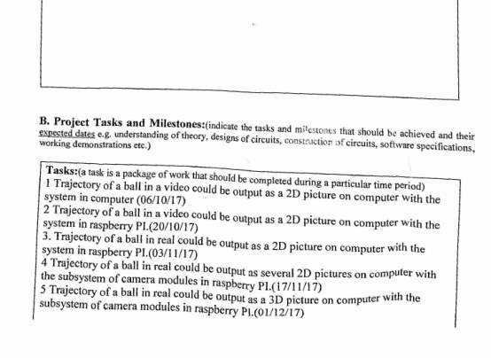
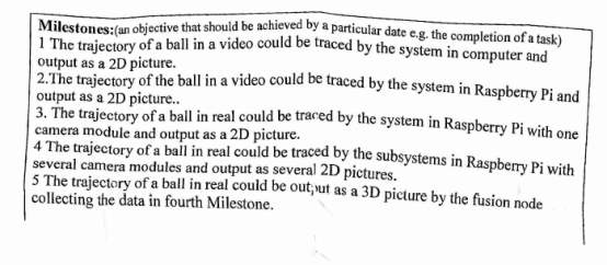
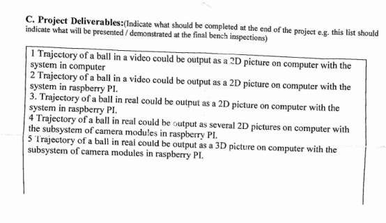
The target of this project was to construct a system comprised of multiple subsystems to trace the movement of a ping-pong ball associated with court lines and the relationship of lines and the path of the ball could be extracted from a three-dimensional space. The scope of this project was image processing and one algorithm of machine learning, that is, Viola-Jones object detection framework. According to this goal, this project could be launched by four steps. Firstly, the two-dimensional movement of a table tennis ball in a video could be recorded and depicted. Secondly, the two-dimensional movement of the ball in real-time would be traced and drawn by one subsystem composed of a Raspberry Pi and a camera module. Thirdly, six two-dimensional routines of the ball would be the output from six symmetrically positioned subsystems like the one in second step. Fourthly, a three-dimensional routine of the ball would be portrayed by a system built upon the six subsystems.
Viola-Jones framework by which human face could be detected was invented by Paul Viola and Michael Jones in MIT at 2001 when it comes to the previous work in object detection [1]. Even though it was originally used in human face detection, its AdaBoost method could also be implemented in general object detection such as airplane detection proved by Ben Weber [2].
With respect to tracing a ball, a process and methodology has been demonstrated by Adrian [3]. Since the capture of scene in different frame and the demand of three dimensional output, then the experience of feature matching would be needed to resolve the position matching problem between frames.
4. Industrial relevance, real-world applicability and scientific/societal impact
This project was an application of computer vision in tracking where the object was a ping-pong ball. The inspiration of this task originated from a goal-line technology named Hawk-Eye computer system. Behind the Hawk-Eye system was the triangulation theory, which exploited images data in time captured by six or more high-speed cameras. These cameras would be symmetrically allocated on-site so that the ball could be detected from various angles. The pixels of the ball on each frame would be recognized by the system and the two-dimensional position of the ball could be identified in real time. Then three-dimensional representation of the ball path would be generated by analysis and combination of all data from subsystems [4]. The general working process of this project was similar to the one of Hawkeye as it was inspired by this cutting-edge tracing technology. Hence, meanwhile, in terms of industrial relevance, the original model of this project was Hawkeye system as well.
From the perspective of circumstances of this application, Hawkeye have been utilized in football, cricket and tennis etc. In the field of football, it has been chosen to serve as the goal-line technology for all matches at EURO 2016 hold by UEFA which is the European administrative institute for football [5]. The Hawk-eye products have been granted a FIFA license for goal-line technology which would be used widely in not only regional scale matches like Italian, English and German leagues but also world-scale competition like 2015 Women’s World Cup hold in Canada [5]. It was mainly used for observing the goal line and judging whether a ball has rolled across the boundary or not. In the field of cricket, the first usage of Hawkeye was a test cricket match between England and Pakistan in 2001 and then it has been extensively used by testing leg-before-wicket decisions [6]. Any kind of spin, swing and bounce could be recorded with 99% accuracy [7]. Meanwhile, a virtual cricket pitch and the excursion of the ball could be represented in three dimensional visualization [7]. In the field of tennis, the system has been employed in many top-level tournaments and the Grand Slams like the 2007 Australian Open, 2007 Dubai Tennis Championships and Tennis Masters Cup [6]. Due to the huge data of match and performance of players it collected, the three dominant bodies of tennis like ATP, WTA and ITF has been assembling data from the product and forming the commercial partner with the company which enjoyed the ownership [8]. Besides, this technology has also been used in snooker, rugby and other ball matches as well with adaptation. All in all, these cases proved the broad applicability of this technology in reality for sports.
Furthermore, the reasons for installing Hawkeye system could be comprised of further improvements for coach to train players, the limitation of vision of referees, and the commercial usage in broadcasting. From the angle of coaching, there are some shot analysis like accuracy of shots, statistics on shots bouncing in intended regions, classification of spins and difference between rising and dropping of ball when crossing the court line. Meanwhile, the speed analysis was offered as well, including the speed of a ball at baseline, apex or the net [9]. These ball tracking details could be investigated for improvement of match performance of athletes. For instance, 2022 China’s winter Olympic national teams’ training would be served by the Hawkeye technology as it was officially claimed [10]. Regarding the function as the assistance of a referee, it would help detect the ball in the accuracy of a millimeter and an alert would be triggered if a ball crosses the goal line and the watch of a referee would receive a vibration and visual signal. The whole process would be finished within a second. This application in all 20 Premier League stadiums would enhance the justice of tennis and cricket matches [11]. From the aspect of broadcasting, it was firstly used by Channel 4 in England [12]. This helped commentators to go back and analysis Hawkeye routine to decide whether the call should have been overturned or not [12]. Meanwhile, it attracted the people watching the game interested in study of players’ techniques and convinced them of the justice of the match. Due to these three achieved functions, the profit rose up as well. The income of Hawkeye technology has risen from 3.3 million pounds to 4.4 million pounds from 2014 to 2015[13].
However, some controversy has been raised especially in the accuracy and job market. Firstly, sometimes the determination of the system could be wrong. The operation of Hawkeye depended on the frames captured by some cameras. On the one hand, the routine of the ball between frames could be purely estimated by the system since the frame rate of the camera would lead to the loss of the position of the ball in every moment. Especially when the ball flies very fast as the record of Murray who could serve a ball at 143 miles per hour [14]. On the other hand, the measure of uncertainty by which the estimation could be calculated has not been provided [14]. Hence, the non-transparency process would cause the doubt of the fairness. Secondly, the replacement of Hawk-eye technology over line judges has been settled down by ATP tennis officials for the events since Gen Finals in Milan November 2017 [15]. This might risk the future of umpires afterwards. Once the Hawkeye technology would be more enhanced and the price of it could be deceased due to the mass manufacture and decreasing value of materials, the possible result will be that Hawkeye technology would be a substitute for all referees in ball matches and a number of people will lose their job. However, these referees could be trained again to be master to interpret the useful information of data collected and still be assistant for the umpire to prevent some mistakes made by the system. Therefore, the social impact probably be negative in the job market but it would still improve the efficiency of training of players.
5. Theory
5.1 Theory of court line detection
Behind the court line detection is Hough line transform. Any straight line could be expressed not only in Cartesian coordinate system but also polar coordinate system. For the elaboration of transform theory, the polar coordinate system is employed. The reason is that when the line is x=a (an arbitrary number) where y is flexible on the line so that it could not be represented by y=mx + a [16]. The situation could be circumvented by polar form. The polar expression for a straight line is
y=-cosθsinθx+(rsinθ)(1) [16]. The parameters are r and
θ. The graphical explanation is demonstrated by the figure (1) below.
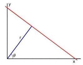
Figure (1) a straight line in a polar coordinate system.
Therefore, with the further arrangement of expression (1), the straight line could be represented by
r=x cosθ+y sinθ(2) where r refers to the distance between the origin to the straight line and
θrefers to the angle between the horizontal axis and perpendicular line of the straight line passing original point [16]. According to equation (2), deduction could be produced that for each fixed point (x0, y0), there are countless lines with different pairs of (r,
θ) passing through the point. Therefore, in terms of a fixed point (x0, y0), a series of lines passing through it could be secured. The relationship between r and
θcould be illustrated by figure (2).
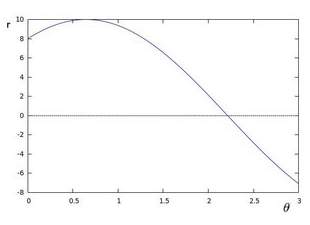
Figure (2) countless pairs of (r,
θ) according to a fixed point (x0, y0)
The case discussed above is only about one fixed point (x0, y0). If there are 3 points (x0, y0), (x1, y1) and (x2, y2) with (r0,
θ0) accidently applicable for these three fixed points, that is, an intersect point of three r-
θcurves drawn in figure (3). The number of intersected r-
θcurves refers to the number of fixed points on a same line [16].
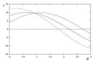
Figure (3) 3 points passed on a straight line.
If there are n points in the picture intended to be tested, there are n r-
θcurves depicted. The more curves intersects at one fixed point, the more points are seated at a same line. Hence, a line could be identified by the manually pre-defined minimum number of intersections between r-
θcurves, which could be interpreted as a threshold [16].
5.2 theory of corner detection
Features are defined in the field of computer vision as characteristics in the different frames of an environment. A corner is one kind of the image features along with edges and blobs[17]. A corner is an intersection of two edges so that at this point, a high variation exist in the corner. Hence, the variation could be utilized as a threshold to define a corner.
In order to find the variation in gradient of image, a sub-window is utilized and moved around the image. The variation of intensity would be calculated when it is sliding over the image. The variation is calculated by the equation:
Eu,v=∑x,yw(x,y)[Ix+u,y+v-I(x,y)]2(3). The window at point (x, y) is represented by W(x, y). The intensity at (x, y) is I(x, y) and the intensity at a moving window (x+u, y+v) is I(x+u, y+v).
The formula (3) could be developed further by Taylor expansion so that
Eu,v≈∑x,yIx,y+uIx+vIy-Ix,y2where the gradient at (x, y) was (Ix, Iy) . Afterwards, the equation could be expressed as
E(u, v)≈∑x, yu2Ix2+2uvIxIy+v2Iy2. If the expression is shown in a matrix form then
Eu,v≈[uv](∑x,ywx,yIx2IxIyIxIyIy2)[uv]. If the term
∑x,ywx,yIx2IxIyIxIyIy2could be denoted as M which is structure tensor of a pixel, the formula (3) ultimately could be
Eu,v≈[uv]M[uv](4)[17].
A score is used as a threshold for determining whether there is a corner in the window or not. It is calculated by two eigenvalues of matrix M, that is, λ1 and λ2. The score is denoted as R.
R=detM-k(traceM)2
(5) where
detM=λ1λ2and
traceM= λ1+λ2. Only windows with the score exceeding R could be considered corners inside. The relationship between two eigenvalues and the pixel is illustrated below as figure (4) where
λ1 and λ2are represented by α and β respectively.
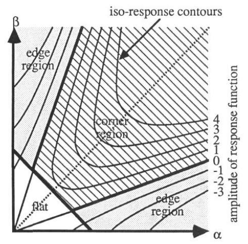
Figure (4) relationship between eigenvalues and region of Harris corner detection.
The contours of score function are drawn and there are three cases depicted on the graph (4). Only the areas are identified as corners in which the score values are positive and other regions would be considered as ‘non-corner’. The first case was that when there are eigenvalues small enough, the pixel is at the ‘flat’ area. The second case is that when only one of two eigenvalues are large enough, the pixel is seated at ‘edge’ area[17]. The third one is that when both of them are large, the pixel would be identified as a corner.
Furthermore, there is an improvement detect method developed from Harris corner detector, that is, Shi-Tomasi Corner detection. Not like the Harris corner detection, the criteria of Shi-Tomasi is determined by
R=min(λ1, λ2)[18]. Then the relationship between eigenvalues and pixel region could be drawn as figure (5).
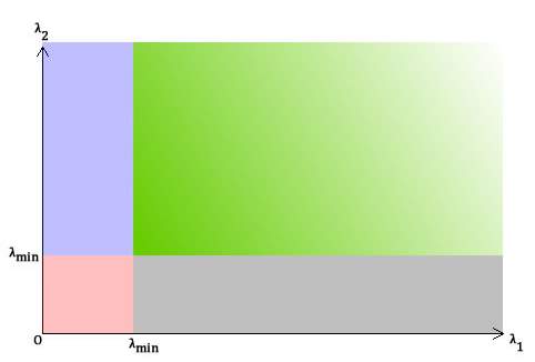
Figure (5) relationship between eigenvalues and region of Shi-Tomasi corner detection.
Similar to the analysis for figure (4), the green area refers to the ‘corner’ pixels. Both purple and grey area are considered as ‘edge’ regions and the red region refers to the ‘flat’.
5.3 Theory of trace of a ball
In terms of the tracking ball, 3 methods could be applicable, that is, Viola-Jones object detection framework, Hough circle detection and colour detection.
5.3.1. Viola-Jones object detection framework.
The viola-jones object detection framework is composed of five stages, that is, collection of data, selection of Haar-like feature, creation of an integral image, training with AdaBoost and cascading of classifiers. Even though it is initially used for face detection, the framework could also be used for general object detection.
The preparation part of the framework is data collection. The data could be collected from video sequences and images. There are two type of data sources, positive and negative images. The positive data set refers to the images where only the object intended to be recognized is included. These pictures of objects should be taken from distinct angles, diverse scales and with various light intensities by which the accuracy of detection could be enhanced [19]. To assure the high training quality, the positive samples should be actual existed samples since the training result would be negatively influenced by any manual modification such as circumvolution by which a large amount data set could be created from a small amount of one. The negative data set could be extracted from the images which contained everything which are not intended to be detected. There are two means to create a set of negative samples. The first approach is that the pictures of background at the place could be taken where the object would be detected by this system. The second idea is that the positive examples could be reused after the object contained region of it has been removed with the rest pixels in grey scale[19].
The second part is the selection of Haar-like features. This name originated in the analogy between a feature and Haar wavelets. The focus of the feature are neighbouring rectangular areas at a certain position in a frame for a detection. The pixel intensities in each area and the difference of these sums would be calculated and these differnce would be used to classify different part of a image. The two main reasons for using Haar-like feature instead of value of pixels were that, firstly, features could be used to cipher specific field expertise that is demanding to be studied by a limited number of training data and secondly. For a system, operation for features could be faster than the calculation of pixels [1].
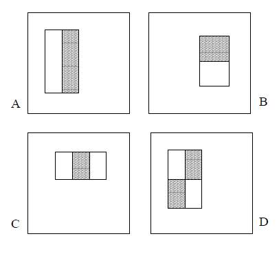
Figure (6). Four basic features for Haar-like features.
There are four basic Haar-like features in Figure (6). Same shape and size are shared by these contiguous rectangles which jointly forms a feature. For the feature combined by two rectangles like the examples in Figure (6) A and B, every feature owns a single value which is calculated by the sum of value of pixels of the black rectangle region subtracting the one in white rectangle area. In terms of the feature composed of three rectangles like figure (6) C, the value of this feature could be obtained by subtracting the sum in two outside regions from the one of the centre region. In terms of the feature comprised of four rectangles like figure (6) D, the value of this feature is calculated by subtracting the sum of value of diagonal pair of white region from the one of black region.
Once the basic features are fixed, then they could be applied to the image where the object would possibly be detected. However, there are only certain critical features to be used to identify an object which meant it is not inevitable to calculate all the feature in the scanned image. For instance, for most of time in the detection of the face, the area of eyes are darker than the upper check and forehead. So it could be depicted by a three-rectangle feature similar to figure (6) C spinning for ninety degree in counter clock direction. Another example is that the bridge of a nose generally looks brighter than the eye area which could be identified by a three-rectangle feature as well such as example (6) C in which white and black areas have been swapped.
Even though a 24X24 sub-window is small, there is more than 170,000 features[1]. For calculation of value of each feature, the sum of the pixels in black and white areas are needed.
To save the calculating time, the new representation called integral image is demanded. The integral image is utilized as an effective way of calculating not only the sum of values in a given image but also average intensity of it. The value at arbitrary point is the summation of all values of pixels above and to the left of (x, y) which is illustrated in figure (7)[20]. The points could also be called as array references.
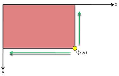
Figure (7). A basic integral image
According to the calculation method in figure (7), if figure (8) was the original picture, then figure (9) is the integral image of (8). The value of pixel at (x,y) of original image is denoted as i(x,y) and the value of an integral image at location (x,y) is denoted as s(x,y).
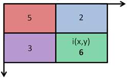
Figure (8). An example of original image.
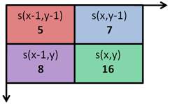
Figure (9). The integral image of figure (8)
The formula for the value of each summed point value is
sx, y=ix,y+sx-1,y+sx, y-1-s(x-1,y-1)(6). In terms of this example, i(x, y)=6, i(x-1,y)=3, i(x-1,y-1)=5, i(x,y-1)=2. Hence, s(x-1,y-1)=i(x-1,y-1)=5, s(x-1, y)=s(x-1,y-1)+i(x-1,y)=5+3=8. S(x,y-1)=s(x-1,y-1)+i(x,y-1)=5+2=7.
S(x,y)=s(x-1,y-1)+i(x-1,y)+i(x,y-1)=16. Since i(x-1,y)=s(x-1,y)-s(x-1,y-1) and i(x,y-1)=s(x,y-1)-s(x-1,y-1), s(x,y)=s(x-1,y-1)+{s(x-1,y)-s(x-1,y-1)}+{s(x,y-1)-s(x-1,y-1)}=s(x-1,y)+s(x,y-1)-s(s-1,y-1) which proves the correctness of equation (6). After rearrangement of equation (6), there is
ix,y=sx-1,y-1+sx,y-sx,y-1-sx-1,y, which would be simplified as
ix,y=sA+sD-sB-s(C)(7) in figure (10). This meant only four variable are needed to calculate a sum of values over an area [20]. Meanwhile, there is another expression for recurrences,
sx,y=sx,y-1+i(x,y)with
iix,y=iix-1,y+s(x,y)where the s(x,y) refers to the cumulative sum of the row of (x,y).
Figure (10). The simplified notation for simplified equation (7).
The advantage of integral image is efficiency. The time used to compute feature is not determined by the size of the image but the number of array references and conversion time of an original image to an integral image.
The training of AdaBoost is the fourth part which is an alternative term for adaptive boosting. [21]. The definition of a classifier is an algorithm by which a classification was implemented. Since this algorithm is used to divide an amount of data and category different set of them, AdaBoost is also a classifier. Boosting is a method to create a strong classifier among weak classifiers to improve the accuracy of algorithms. The goal could be achieved by extraction of a model from data and creation of a second model by which the faults of the first one could be corrected [22]. Hence, adaptive boosting meant a boosting algorithm which could be adjusted by itself in different situations.
The analogy of AdaBoost could be elaborated by a task to find all people in a town who is shorter than 1.5m, weight less than 50kg, and the age range of them should be between five to fifteen. The people who are aimed to be found could not be determined by only one factor, that is, one classifier. That’s why these three parameters have to be estimated by three classifier separately and the result of the task should be a combination of determination of these three factors.
However, since strong classifiers demands a huge number of potential features which could lead system operation to run slow, these affordable classifiers are weak ones. To improve the performance of classification, cascade method was used on these weak classifiers. These weak classifier would be cascade together to form a strong classifier. During the cascading process, there are lots of learning rounds to identify different features [21]. If the frequency of wrong identification by a classifier increased which means the accuracy of the classifier is low, then the weight of other classifier could be increased and the weightage of this easily fallible classifier would be given less in the following cascading [21]. Overall, after several rounds of cascading, the accuracy would be improved.
Into the details of operation of AdaBoost to learn features in image, a classification function could be learned by the AdaBoost with a set of feature, a group positive and a group of negative images. In this case, the AdaBoost is used for not only selection of features but also training of the classifier. The original function of AdaBoost is utilized in order to improve the performance of a weak learning algorithm. Because the number of features linked with each sub-windows is larger than the number of pixels, the process of whole set would be time-consuming. To improve the efficiency of computing feature, some unnecessary features would be abandoned since only a small set of features is required to produce an effective classifier [1].
In order to obtain the useful features, the weak learning algorithm is constructed to choose single feature by which the positive and negative images are distinguished efficiently. Regarding every feature, the superlative threshold classification function would be produced so only few number of them would be classified wrongly. For weak classifiers, when
pjfjx<pjθj,
hjx=1and when
pjfj≥pjθj,
hjx=0where fj ,
θj,pjreferred to a feature, a threshold and a parity respectively [1].
The boosting process of AdaBoost in selecting useful features could be summarised as two premises and four steps. The first condition is that image of both negative and positive examples have been given such as (x1, y1), (x2, y2), …. (xn, yn). The second condition is that weights would be initialized like
w1,i=12mwhere m represented the number of negative images and
w1,i=12lwhere l refers to the number of positive images. Both premises are given under the condition that
yi=0,1In the case of t varies from 1 to T, the first step is that weights should be normalised.
wt,i←wt,i∑j=1nwt,j. In terms of feature, j, a classifier hj where only a single feature is used. The evaluation of the error is related to wt and hence the formula of the error is
∈j=∑iwi|hjxi-yi|. The third step is that the classifier ht where lowest error
∈jexists would be chosen. The fourth step is that the weights of different classifier would be updated. The reweighted by
wt+1,i=wt,iβt1-ei. When the example xi is classified correctly,
ei=0. When it is classified incorrectly,
ei=1. After these four steps, eventually, the strong classifier is
hx=1when
∑t=1Tαthtx≥ 12∑t=1Tαtand
hx=0when
∑t=1Tαthtx< 12∑t=1Tαtwhere
αt=log1βt[1]. During boosting in early rounds, only features where error rates are in the range of 0.1 to 0.3 would be selected. In the later rounds, features with error in the range of 0.4 and 0.5 would be chosen[1].
5.3.2. Hough circle detection
Hough circle detection could be utilized since the object in this project is a tennis ball which was a circle in every frame. The circle Hough transform is the elemental approach for this detection. In the two-dimensional Cartesian coordinate system, the formula of a circle is listed below.
r2=(x-a)2+(y-b)2
(8)
In this formula, a, b, r refers to the position of the centre and radius of the circle respectively. The alternative expressions are below.
x=a+r*cos(θ)
(9)
y=b+r*sin(θ)
(10)
Unlike the Hough transform of a straight line detection, circular one depends on three parameters, that is, a, b and r. When r of a circle Q equals to a fixed number R and the centre of it in the geometric space was A(x1,y1), three-dimensional parameter space a,b,r turns into a two-dimensional space a and b [24]. For instance, there are three pairs of (a,b), that is, B(a1,b1), C(a2,b2) and D(a3,b3) in the space of parameter, the intersection of new circles whose centres were B, C and D with fixed radius R would be the point A in parameter space. Because there are countless points on the circle Q instead of only B,C and D, if these points are set as centre points of circle in parameter space with the radius of Q, then the numerous new circles in the parameter space would intersect in point A as well. The times of a point like A being passed through by n circles would be counted as n (n is an arbitrary integer) which is a procedure of voting . The points which would be counted most in the image would be identified as a centre of the circle aimed to be detected [24]. This situation is drawn in the figure [11] with the geometric coordinate system in the left and the parameter coordinate system in the right [25].
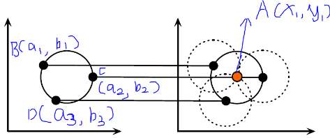
Figure [11]. The case with fixed r in Circular Hough Transform.
5.3.3. Colour object detection
In terms of human vision, the achromatic light refers to a light without colour like gray scale and chromatic light refers to the visible lights on the electromagnetic spectrum [26]. the cone receptors is in charge of chromatic light and rods receptors is responsible for achromatic light in the human eye [27]. Three types of cone receptors could detect short-wavelength, meddle wavelength and long wavelength colours, that is, blue, green and red in Trichromatic theory [28]. The sensitivities of reddish, greenish and bluish colour could be measured as three varieties. However, these varieties overlap each other in the realm of wavelength in the diagram [12] of wavelength related to relative sensitivity depicted below. Hence, the limitation of the Trichromatic theory is that the monochromatic colours like orange could not be exactly duplicated since the wavelength of it falls only in reddish and greenish spectrum while the overlap of them in frequency contains the bluish stimulus which could impede the reproduction of pure orange. Nevertheless, the issue of the replication of pure colours could be resolved by signal processing technology so that the Trichromatic theory is still acknowledged with red, green and blue as standard primitive colours in colour representation officially.
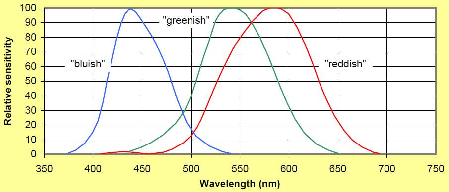
Figure [12]. The wavelength and sensitivity relationship of colours.
In terms of digitalized representation of colours, all colours could be characterized by the value of their hue, saturation, intensity and brightness value. Hue refers to the predominant wavelength of the colour, that is, one of red, green, blue, yellow, orange and violet [29]. Saturation determines the lighting condition of the colour, from no white to full white, referring to the intensity of the colour [30].Brightness meant the intensity of black in the colour [31]. However, the effect of increasing value of the brightness doesn’t equal to the one of decreasing value of saturation. The saturation only affects the level of intensity of the colour which reflects the degree of grey while the brightness only affected the intensity of black [31]. The difference could be better understood by the figure [13].
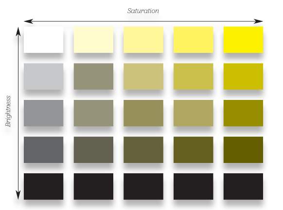
Figure [13].different effect of brightness and saturation.
When it comes to the colour model in this project, RGB facilitates colour representation in digital photography as a number by a mathematical equation. It is an additive colour model to form various colours by primary colours, that is, red, green and blue. The model is created in an unit cube with three-parameters coordinate system (R, G, B). The plane is drawn below as figure [14].
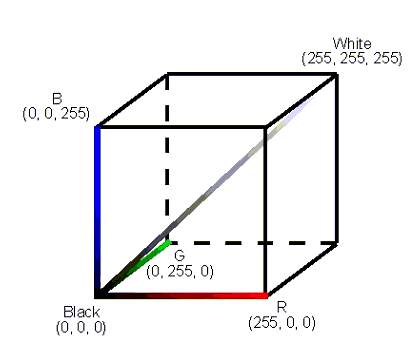
Figure [14]. RGB model cube
The range of these three parameters are from 0 to 255. If the parameters are all zero, it refers to black. Conversely, if the parameters are all 255, it refers to white.
Even though RGB could be employed for computers, it is not user-friendly so that other colour models like HSV/HSB and HSL were invented to facilitate colour specification in programming. In terms of the name of the models, H refers to hue and S was noted as saturation. The HSV was another name for HSB since V refers to value of the brightness and B refers to brightness as well. So the main difference is between HSV and HSL. The definition of H in HSV and HSL both refers to the hue. However, the S, that is, saturation would be calculated in different way. L meant lightness which was different from the definition of brightness. Lightness meant the amount of light on white while brightness was interpreted as the amount of light for arbitrary colour.
For the calculation of H from RGB to HSV, firstly, the range of RGB should be rearranged into range [0, 1] by following equations [32],
R’=R/255
,
G’=G/255
,
B’=B/255
.
Secondly, the difference between the maximum value and minimum value of (R’, G’, B’) is obtained by the following equation [32].
∆=maxR’,G’,B’-min(R’,G’,B’)
H=0o, if ∆=060o*G-B∆mod6, if Cmax=R’60o*B-R∆+2, if Cmax=G’60o*R-G∆+4, if Cmax=B’
For the calculation of S from RGB to HSV,
S=0, if Cmax=0 ∆Cmax, if Cmax≠0
In terms of the conversion of V from RGB to HSV,
V=Cmax..
When it comes to conversion from HSV to RGB, then the values could be obtained by following equations when H is in the range of [0,360], S and V are both in the range [0,1] [33].
C=V*S
X=C*(1-|H60omod2-1|)
m=V-C
R’,G’,B’=C,X,0, 0o≤H<60oX,C,0, 60o≤H<120o0, C,X, 120o≤H<180o0,X,C, 180o≤H<240oX,0,C, 240o≤H<300oC,0,X, 300o≤H<360o
R,G,B=(R’+m*255, G’+m*255,B’+m*255)
6. Design
According to the three dimensional space requirement of this project, the hardware was intended to be six subsystems symmetrically positioned around a tennis table to assure a precise trace. Each subsystem consist of one Raspberry PI model and a camera module. In the plan, after successful construction of subsystems, a fusion node would be set up on the basis of six subsystems. Regarding to the software design, the functions of detection of lines, corners and the ball should be separately. However, in the first place, an appropriate interface development environment should be adjusted with OpenCV library with additional download of packages like numpy. In reality, even though python and c++ could both applied to this project, it is more convenient to code in python on the platform of Pycharm especially when it comes to download lots of packages with no further compatibility issue between the library and the IDE.
7. Experimental method
The experimental method associated with the hardware is the installation of NOOBs which is the operation system of Raspberry Pi, the installation of OpenCV library and related packages. Firstly, a formatted SD card is needed to save the NOOBs file. A 32GB SD card was chosen since free space of the SD card has to be more than 8GB to accommodate the size of the system and downloaded packages. Secondly, a power lead is needed for offering power to Raspberry Pi board. Thirdly, a monitor and a HDMI line are demanded for displaying the PIXEL Linux desktop. Fourthly, a mouse and a keyboard are acquired for interaction. No more USB hub is required since there are two ports in the Raspberry PI 3 model which support wireless internet connection enough for one USB flash drive and a HDMI line.
From the perspective of programming, in terms of the detection of lines, Hough line transform was used. In terms of the detection of corners, Shi-Tomasi corner detector was used. The strategy for improving accuracy of both was to modify parameters and compare the results.
In terms of the ball detection, the Haar-like feature cascade classifier, the color detection and Hough circle transform were used separately. The first one is Haar-like feature cascade classifier training. Due to the Viola-Jones detector was initially used in face detection. The test of face detection had been executed before this project. However, the experimental method of the ball detection as the same as the one of this face detection .
In order to build a Haar-like Classifier, six steps are adopted during training.
The first step was the search and collection of two image data sets, positive one and a negative one. 200 positive and 200 negative images were gathered. Only faces contained in the positive samples were shown as figure[15].Non-faces objects included in the negative samples were shown in figure[16].
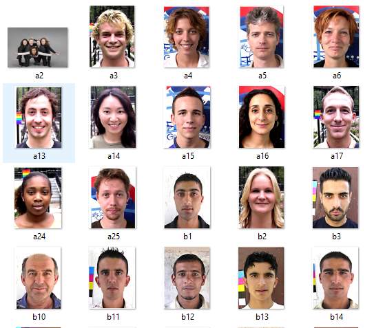
Figure[15]. arbitrary selection in positive data set.
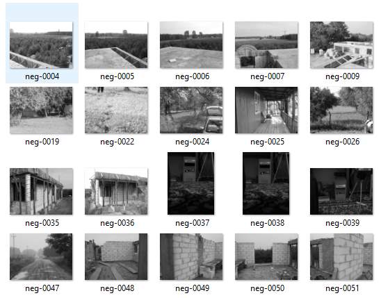
Figure[16]. arbitrary selection in negative data set.
The second step was to create a description file for negative images. Basically, it is a text file listing all image file name from the first negative image to the last one. For instance, the first line is”neg-00001.jpg” and the last line is “neg-0200.jpg” which indicates there were 200 images in the file called “negative” with the rule that each file name occupies a line. The path of the description file of negative images was also the one of all the negative images. This text file could be created by typing all the image name in a new text file or, more convenient, in this case, running a batch file called “create_list” which can automatically output the required text file. Eventually, the view of folder of the negative images would be like the figure[17] below.

Figure[17]. The negative images, negative description file”bg.txt” with the generation batch file in “negative” folder.
The third step was to yield the more precise object ranges of pixels based on every positive images. Since a vector file of positive samples is needed for training, which was similar to the description file of negative image, the objects in the positive images had to be marked by cropping in the picture window. Firstly, a exe file called “objectmaker” would be operated to mark all positive images in turns with the assistance of “highgui.dll” and “cv.dll” in the same directory. After this file was clicked, then two window appeared. One was the positive image and the other was a command prompt showing the name of this positive image which is about to be cropped. Afterwards, the image could be straightaway marked by clicking at left tip corner of the wanted object to the right bottom corner of it while the left-key of the mouse was always kept down. At the moment the left-key was released, the position of the mouse in the window was marked as the right corner position of the object. Meanwhile, the position, width and height of the object in the frame would be displayed in the command prompt which would be stored in the text file named “info.txt” simultaneously. Sometimes there were multiple faces in one image so that every face needed to be cropped in turns. The interface is shown in figure [18].
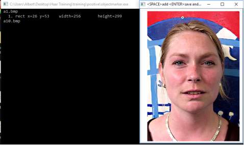
figure[18] Left command prompt window for displaying information of cropped samples in right one.
The fourth step was to create a vector file for the more precise positive data set. A batch file was created, whose content was “createsamples.exe -info positive/info.txt -vec vector/facevector.vec -num 200 -w 24 -h 24”. The first parameter “createsamples.exe” referred to the exe file which would be executed for making this vector. The second parameter”-info positive/info1.txt” meant that the information of cropped positive images was stored in the “info1.txt” file which was in the directory named “positive”. The third parameter “-vec vector/facevector.vec” meant that the produced vector file named “facevector.vec” would be stored in the directory “vector”. “-num 200” indicated that the number of positive images was 200 and “-w 24 -h 24” meant that the width and height of these objects were 24 and 24 respectively. Since the file “createsamples.exe” would take advantage of functions outside, dynamic-link library files like”highgui097.dll” should be included in the same “training ” folder shown in figure[19] and the vector file is shown in figure [20].
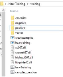
Figure[19]. All files in the folder of “training”.
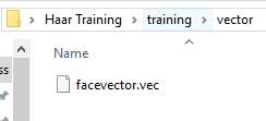
Figure[20]. The vector file of positive data set in the folder of “vector”.
The fifth step was to trigger the Haar-like training process. In the folder of “training”, the content inside the batch file “haartraining.bat” was adjusted as shown below in figure[21].

Figure[21]. The command of batch file “haartraining”.
In this command, “-data cascades” meant that the cascade of classifiers would be stored under the directory named “cascades”. “-vec data/vector.vec” referred to the position of the vector file of the positive data. “-bg negative/bg.txt” referred to the location of the description file of negative data. “-npos 200” and “-nneg 200” meant that both the quantity of positive images and the one of negative images were 200. “-nstages 15” meant that the number of training stages was 15. “-mem 1024” meant that the size of memory space allocated to the training was 1024MB. “-mode ALL” meant that the kind of Haar features set selected in training were the upright total set and 45 degree adjusted one. The training result is shown in figure [22].

Figure[22]. training results in folder of “cascades”
The sixth step was to create a XML file. After the fifth step, in the folder of “cascades” there were catalogues from “0” to “14”, 15 folders which were the results of 15 training stages where there was a txt file called “AdaBoostCARTHaarClassifier” in each one. All the 15 folders would be moved into the in the folder “data” in “cascade2xml” of the location “C:UsersAlbertDesktopHaar Training”.
The same process applied to the ball detector training with only the difference of parameters which are number of positive and negative samples. There were 196 negative samples and 50 positive samples. The produced xml file is shown in figure[23].
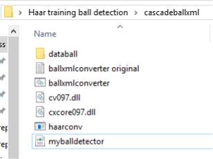
Figure[23].The XML result of ball detection.
8. Results and Calculations
From the angle of hardware result, problems of creation of python-opencv environment appeared many times with different issues as figure [24] shown.
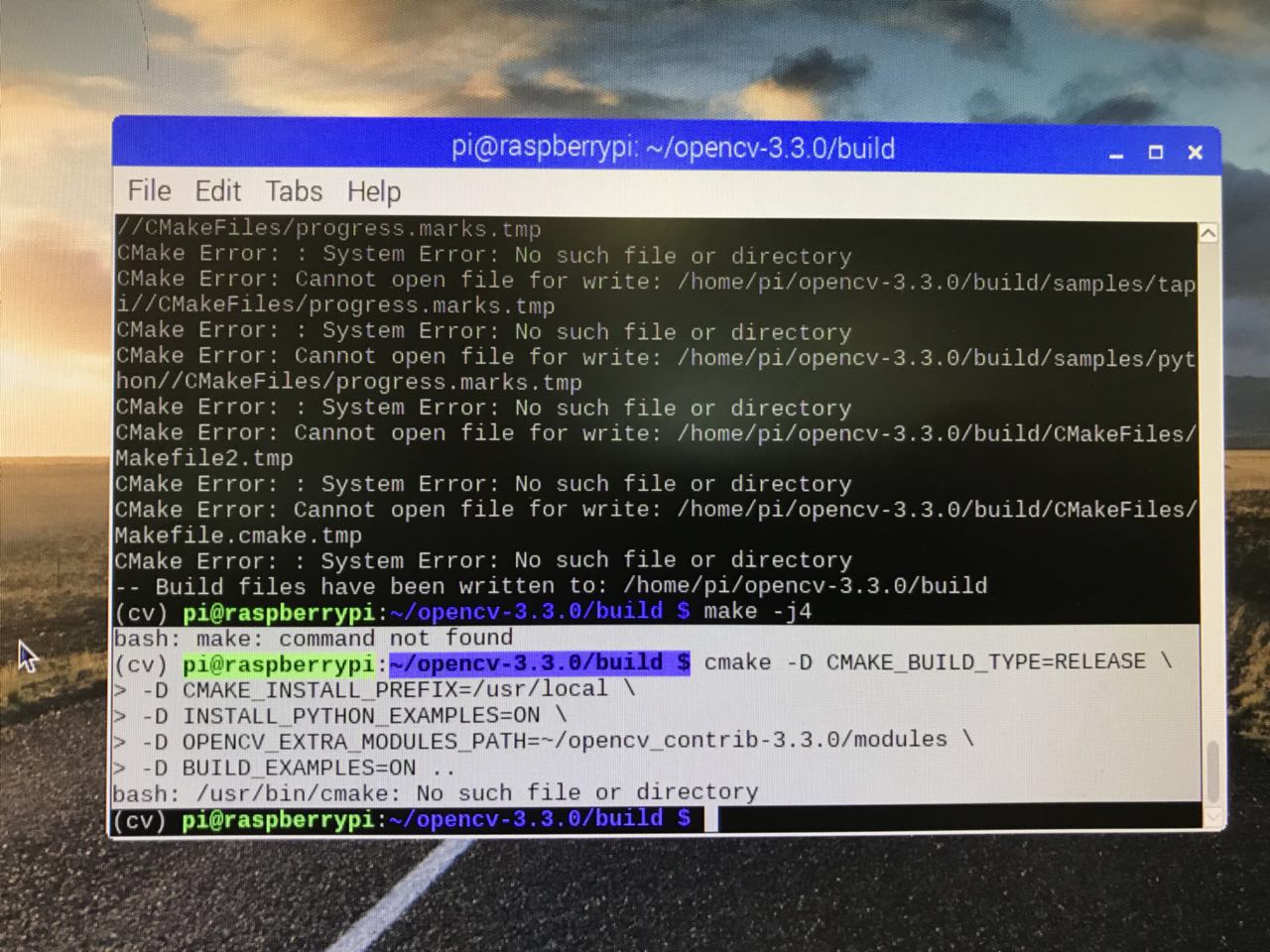
Figure[24]. Screenshot of the failure of compiling OpenCV on Raspberry PI
The code of face detection was show below.
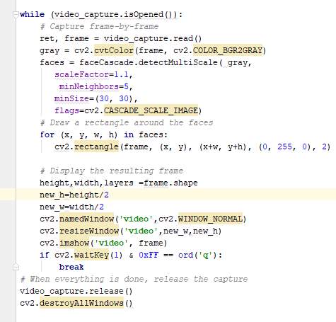
figure[25].The code of face detection.
The face training result was shown below.
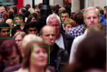
Figure[26]. the result of face detection as a test of Haar-training model.
The result of line detection and corner detection were shown below as figure[27][28].
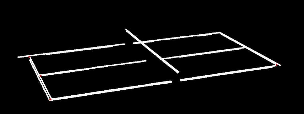
Figure[27]. The result of line and corner detection.
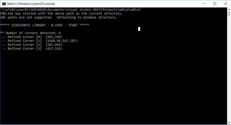
Figure[28]. The position of corner detection.
The result of ball detection by Haar-like cascade training result was shown as figure[29].
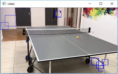
Figure[29].Result of detection of the ball by Haar-like training.
The result of ball detection by color detection was listed as figure[30].
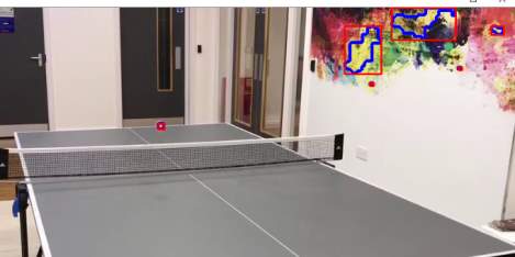
Figure[30].Result of detection of the ball by color detection.
The result of ball detection by circle detection was listed as figure[31].
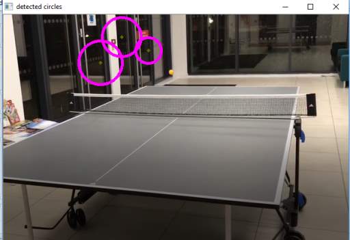
Figure[31]. Result of detection of the ball by circle detection.
9. Discussion
In the Hough Circle detection, an artificially set value of the fixed radius in advance would influence the detection result since not only position of the object on the image but also the distance between the object and the camera would led to the inaccuracy of the detection.
The possible reason for why the ball detector of cascade training cannot detect the ball correctly in the video frame was that the positive and negative samples are not enough. Besides, the feature of a ball was not as obvious as human face having a distinguished dark and bright part like upper cheek and eyes. It would be hard for the classifier to learn.
10. Conclusions
In conclusion, regarding to the preparation, since the convenience of adjustment between Pycharm and OpenCV and there was already Python IDE on the raspberry PI, the python should be chosen as the language instead of C++ at the beginning of this project.
in terms of object detection in machine learning way like Haar-like feature cascade training, the number of samples of positive and negative images should be more than two hundreds. The objects in positive samples should be under different angle and lighting conditions instead of the one in the video which is used to test.
11. References
Online materials:
[1] Rapid Object Detection using a Boosted Cascade of Simple Features[Available] http://wearables.cc.gatech.edu/paper_of_week/viola01rapid.pdf
(Accessed: 13th, April, 2018)
[2] Generic Object Detection using AdaBoost [Available] https://pdfs.semanticscholar.org/presentation/b10b/365912ba4bdb6decd9dc684bcedc3074d077.pdf
(Accessed: 13th, April, 2018)
[3] OpenCV panorama stitching [Available] https://www.pyimagesearch.com/2016/01/11/opencv-panorama-stitching/
(Accessed: 13th, April, 2018)
[4] Hawk-eye Line-calling system. [Available] https://www.topendsports.com/sport/tennis/hawkeye.htm
(Accessed: 13th, April, 2018)
[5] Hawk-eye to deliver goal line technology for UEFA EURO 2016 [Available]https://www.hawkeyeinnovations.com/news/45525
(Accessed: 13th, April, 2018)
[6] Which sports use Hawkeye?[Available] http://www.stpetersbray.ie/piinthesky/which-sports-use-hawkeye/ (Accessed: 13th, April, 2018)
[7] How does Hawk-eye work? [Available] http://news.bbc.co.uk/sportacademy/hi/sa/cricket/features/newsid_3625000/3625559.stm(Accessed: 13th, April, 2018)
[8] unlocking hawk eye: what it means for tennis, the ATP, WTA and ITF [Available] https://channels.theinnovationenterprise.com/articles/unlocking-hawk-eye-what-it-means-for-tennis-the-atp-wta-and-itf(Accessed: 13th, April, 2018)
[9] Smart Coach for tennis [Available]https://www.hawkeyeinnovations.com/expertise/coaching(Accessed: 13th, April, 2018)
[10] Hawkeye technology to support China’s Winter Olympic training [Available] https://www.chinadaily.com.cn/m/beijing/zhongguancun/2017-01/23/content_28031756.htm(Accessed: 13th, April, 2018)
[11] English Premier League to integrate cameras to help referees with goal-line calls [Available]https://www.theverge.com/2013/4/11/4212432/epl-will-use-hawkeye-goal-line-tech-this-year(Accessed: 13th, April, 2018)
[12]The Tech behind Cricket Broadcasting [Available] https://www.gizmodo.com.au/2013/08/the-tech-behind-cricket-broadcasting/
(Accessed: 13th, April, 2018)
[13] Owzat! Profits at company behind ball-tracking Hawk-Eye technology hit £4.4m
http://www.thisismoney.co.uk/money/markets/article-3382128/Owzat-Profits-company-ball-tracking-Hawk-Eye-technology-hit-4-4m.html(Accessed: 13th, April, 2018)
[14] Hawk-Eye at Wimbledon: it’s not as infallible as you think [Available] https://www.theguardian.com/science/sifting-the-evidence/2013/jul/08/hawk-eye-wimbledon(Accessed: 13th, April, 2018)
[15] ‘Hawk-Eye live’ set to launch at next gin ATP finals [Available]
http://www.nextgenatpfinals.com/en/news-and-media/tennis/hawk-eye-live-at-2017-next-gen-atp-finals (Accessed: 13th, April, 2018)
[16] Hough line transform [Available] https://docs.opencv.org/2.4/doc/tutorials/imgproc/imgtrans/hough_lines/hough_lines.html (Accessed: 13th, April, 2018)
[17] Fundamentals of Features and Corners [Available] http://aishack.in/tutorials/harris-corner-detector/(Accessed: 13th, April, 2018)
[18] Shi-Tomasi Corner Detector & Good Features to Track [Available] https://docs.opencv.org/3.0-beta/doc/py_tutorials/py_feature2d/py_shi_tomasi/py_shi_tomasi.html (Accessed: 13th, April, 2018)
[19] Object detection (work-in-progress) [Available] http://melvincabatuan.github.io/Object-Detection/(Accessed: 13th, April, 2018)
[20] Computer Vision – The integral Image [Available] https://computersciencesource.wordpress.com/2010/09/03/computer-vision-the-integral-image(Accessed: 13th, April, 2018)
[21]what is AdaBoost? [Available] https://prateekvjoshi.com/2014/05/05/what-is-adaboost/(Accessed: 13th, April, 2018)
[22]Boosting and AdaBoost for Machine Learning [Available] https://machinelearningmastery.com/boosting-and-adaboost-for-machine-learning/(Accessed: 13th, April, 2018)
[23]cascade classification [Available] https://docs.opencv.org/2.4/modules/objdetect/doc/cascade_classification.html(Accessed: 13th, April, 2018)
[24]Lecture 10: Hough Circle Transform [Available] https://www.cis.rit.edu/class/simg782/lectures/lecture_10/lec782_05_10.pdf(Accessed: 13th, April, 2018)
[25]Object detection using circular hough transform
http://wcours.gel.ulaval.ca/2015/a/GIF7002/default/5notes/diapositives/pdf_A15/lectures%20supplementaires/C11d.pdf(Accessed: 13th, April, 2018)
[26] Color images, color spaces and color image processing
http://www.uio.no/studier/emner/matnat/ifi/INF2310/v17/undervisningsmateriale/slides_inf2310_s17_week08.pdf(Accessed: 13th, April, 2018)
[27] a review of rgb color space. http://www.babelcolor.com/index_htm_files/A%20review%20of%20RGB%20color%20spaces.pdf(Accessed: 13th, April, 2018)
[28]understanding the trichromatic theory of color vision.
https://www.verywellmind.com/what-is-the-trichromatic-theory-of-color-vision-2795831(Accessed: 13th, April, 2018)
[29]The ultimate guide to understanding hue, tint, tone and shade.
https://color-wheel-artist.com/hue/(Accessed: 13th, April, 2018)
[30]color saturation
https://www.techopedia.com/definition/1968/color-saturation(Accessed: 13th, April, 2018)
[31]difference between saturation and brightness.
https://designingfortheweb.co.uk/part4/part4_chapter17.php(Accessed: 13th, April, 2018)
[32]RGB to HSV color conversion
https://www.rapidtables.com/convert/color/rgb-to-hsv.html(Accessed: 13th, April, 2018)
[33]HSV to RGB color conversion
https://www.rapidtables.com/convert/color/hsv-to-rgb.html(Accessed: 13th, April, 2018)
12. Appendix
The updated Gantt Chart is shown below.
| 20/10/2017 | 03/11/17 | 20/02/2018 | 07/03/2018 | |
| Detect count lines | ||||
| Detect the corner | ||||
| Cascade training | ||||
| Detect the ball |
Cite This Work
To export a reference to this article please select a referencing stye below:
Related Services
View all


Related Content
All TagsContent relating to: "Information Systems"
Information Systems relates to systems that allow people and businesses to handle and use data in a multitude of ways. Information Systems can assist you in processing and filtering data, and can be used in many different environments.
Related Articles

DMCA / Removal Request
If you are the original writer of this dissertation and no longer wish to have your work published on the UKDiss.com website then please: