Simulated Raman Spectral Analysis of Organic Molecules
Info: 7070 words (28 pages) Dissertation
Published: 9th Dec 2019
Tagged: Organic Chemistry
The advent of the laser technology in the 1960s solved the main difficulty of Raman spectroscopy, resulted in simplified Raman spectroscopy instruments and also boosted the sensitivity of the technique. Up till now, Raman spectroscopy is commonly used in chemistry and biology. As vibrational information is specific to the chemical bonds, Raman spectroscopy provides fingerprints to identify the type of molecules in the sample. In this thesis, we simulate the Raman Spectrum of organic and inorganic materials by General Atomic and Molecular Electronic Structure System (GAMESS) and Gaussian, two computational codes that performs several general chemistry calculations. We run these codes on our CPU-based high performance cluster (HPC). Through the message passing interface (MPI), a standardized and portable message-passing system which can make the codes run in parallel, we are able to decrease the amount of time for computation and increase the sizes and capacities of systems simulated by the codes. From our simulations, we will set up a database that allows search algorithm to quickly identify N-H and O-H bonds in different materials. Our ultimate goal is to analyze and identify the spectra of organic matter compositions from meteorites, and compared these spectra with terrestrial biologically-produced amino acids and residues.
1.1 A Brief History of Raman Spectroscopy
2.2 Vibrational modes of a molecule
2.7 High-Performance Computing Cluster
CHAPTER IV: RESULTS AND DISSCUSSION
4.3 Result of Glycine Simulation
4.4 Result of Glycine Aqueous Solution
Table 2: Methane theoretical values and experimental results
Table 4: Water molecule theoretical values and experimental results
Table 5: Glycine molecule theoretical values and experimental results
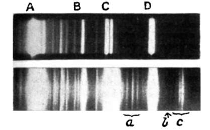
Figure 1: Spectrum of incident light(above) and scattered light(below)
Figure 2: Stokes/Anti-Stokes bands shifted from Rayleigh lines.
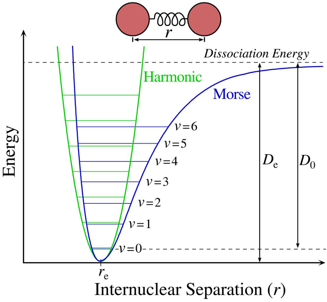
Figure 4: The Morse potential (blue) and harmonic oscillator potential (green) curve.
Figure 5: Amino acid general structure.
Figure 6: Fixed linear combination of Gaussian functions to construct GTO basis.
Figure 7: Illustration of a simulation of lysozyme-water system
Figure 8: Basic components of a HPC cluster.
Figure 9: 3-D model illustrate the structure of methane (CH4)
Figure 10: Fundamental vibrational modes of methane (CH4)
Figure 11: Unscaled simulated Raman spectrum for methane and published Raman spectrum for methane.
Figure 12: Scaled simulated Raman spectrum for methane and published Raman spectrum for methane.
Figure 13: 3-D model illustrate the structure of water (H2O)
Figure 14: Fundamental vibrational modes of water (H2O)
Figure 15: The unscaled simulated Raman spectrum and scaled simulated Raman Spectrum for water
Figure 16: Published Raman Spectrum for water range from 1400-1800cm-1 and 2800-3800cm-1
Figure 17: 3-D model illustrate the structure of water dimer (H2O-H2O)
Figure 19: 3-D model illustrate the structure of Glycine (C2H5NO2)
Figure 20: Simulated Raman Spectrum for Glycine with different basis sets
Figure 21: Simulated Raman Spectrum with ACCD basis set and published Raman Spectrum for Glycine
Figure 22: Illustration of Glycine aqueous solution system
Figure 23: Plotting of RMSD (nm) of glycine solution respect with Time(ns)
Twenty percent of the human body is made up of protein. Protein plays a crucial role in almost all biological processes, including forming orgasmic tissues and building up enzymes to keep our body functioning normally. Amino acids, which are the building blocks of proteins, also play a crucial role in our lives. A large amount of our cells, tissue, and muscles build by amino acids, meaning they perform many significant important bodily functions. For example, in the human brain, glutamate and gamma-aminobutyric acids are, respectively, the main excitatory and inhibitory neurotransmitters [1]. Therefore, the study of amino acids’ biological and chemical properties can help provide a deeper understanding of the origin of life and the production of drugs, biodegradable plastics, and chiral catalysts.
Due to the fact that an amino acid is a small molecule, a proper tool is needed to study its properties. Raman Spectroscopy is exactly the tool to carry out this job.
In 1923, a paper titled “The quantum theory of dispersion” was published in the science journal Naturwissenschaften by the Austrian quantum physicist A. Smekal [2]. This paper theoretically predicted the scattering of monochromatic radiation with a change in frequency of light-material interaction, later called Raman scattering. Scattering light passing through various mediums was studied after the first prediction, but no change in wavelength was observed until 1928, when Indian scientist C.V. Raman and his coworker K.S. Krishnan first discovered this kind of inelastic scattering using a quartz mercury vapor lamp [3]. By comparing the spectra in Figure 1 from the incident light and the scattering light, one sees several other lines in addition to the lines in the incident spectrum. Raman and Krishnan published their finding in Nature with the title “The optical analogue of Compton effect,” and 2 years later they received the Nobel Prize in physics for their observation of light inelastic scattering, which was named Raman scattering in honor of his contribution.
Developments in Raman spectroscopy based on the theory of Raman scattering occurred slowly during the period from 1930 to 1950, since there was no proper monochromatic radiation source. In the early experiments during the 1930s, the mercury lamp, filtered to offer the monochromatic light, was the most common radiation source. The mercury Toronto arc lamp was introduced as the ultimate source later in 1952 [4]. However, the intensity of the mercury arc lamp was so weak that they needed significant exposure time for the photographic receiver to create a readable Raman spectrum. The invention of laser technology in 1960 solved this problem and provided a monochromatic source, which improved the Raman scattering intensity and shortened the time for exposure. In 1962, Porto and Wood [5] reported the first use of a pulsed ruby laser for exciting Raman spectra. After that, Raman spectroscopy developed quickly and became a practical tool for studying vibrational information on the molecular atomic scale in many fields.
The ultimate objective of this thesis is to utilize an advanced computational technique to simulate the Raman spectrum of inorganic and organic material as compelling data for analyzing and identifying the organic components in an unknown sample. Since Raman spectroscopy can provide fingerprints to identify the type of molecules in the sample, it is important to understand the pattern of Raman Spectrum for different organic materials. We start with the simplest amino acid, water and glycine, by using the General Atomic and Molecular Electronic Structure System (GAMESS) which is a quantum chemistry computational code, on our High Performance Computing (HPC) cluster to obtain its Raman spectrum. By analyzing this spectrum, we determine some characteristic peaks that are the fingerprint of glycine and write a search algorithm for identifying a specific kind of amino acid from its Raman spectrum. After we verify the corrective rate of our search algorithm, we set up a database that allows search algorithm to quickly identify N-H and O-H bonds in different materials. Since Raman spectroscopy has some advantageous properties, such as its ability to be used with solids and liquids without the preparation of a sample, it is used widely in mineral identification and characterizations of bio-molecules. If this search algorithm can satisfy the tolerance as expected, it can be applied on a deep space explorer to analyze organic material outside the earth automatically, which can avoid the delay present in long-distance data transition.
In this chapter, we are going to introduce some basic concepts related to our topic. Since the Raman Spectroscopy is a significant tool for our study, it bases on the Raman Scattering effect. So Raman Scattering will be the first section introduced in this chapter. For the next section, vibrational modes of a molecule will be explained. The first two sections 2.1-2.2 are the theory to explain how Raman spectroscopy can determine the unknown matter by the spectrum. For the section 2.3, the basic chemical structure of our research objects, Amino Acids are introduced. For the next two sections 2.4-2.5, the Hartree-Fock method for calculating the simulated Raman Spectrum is presented. In the last two sections (2.6-2.7),both the simulation software we used and the platform for the software are introduced.
When light encounters matter, either absorption or scattering occurs. Infrared spectroscopy based on the absorption process, and the Raman Spectroscopy based on the scattering process.
The process of absorption requires the energy of the incident radiation to be exactly equal to the energy difference between the ground state and the excited state of a molecule. After the molecule absorbs the energy from the incident light, the electron in the ground state jumps to the excited state. Therefore, the spectrum of transmitted light will have some frequency bands are missing. The frequency of the missing band equals to the vibrational frequency of the molecule. By plotting out the intensity of the transmitted light in terms of frequency, one can get the IR spectrum and identify specific chemical groups within the molecule.
In contrast, scattering does not require the incident radiation to match the energy difference between the ground and excited states. As a light wave, considered an oscillating dipole, passes through the molecule, it interacts and distorts the clouds of electrons orbiting the nuclei. Energy is released in the form of scattered radiation. Since the wavelength of visible light is much greater than the size of a common molecule, when the light wave interacts with the molecule the oscillating dipole polarizes the electrons and excites the molecule to a higher energy state called a “visual state.” This transformation acts in a short time; unlike electrons, which have a smaller mass, the nuclei do not have time to respond. This process results in the molecule reaching a high-energy state by changing the electron geometry without moving the nuclei. Since these high-energy-state electrons are unstable and cannot last for a long time, they drop back to their ground state and release photons in random directions. This release light is called scattering radiation.
There are two types of scattering: Rayleigh and Raman scattering.
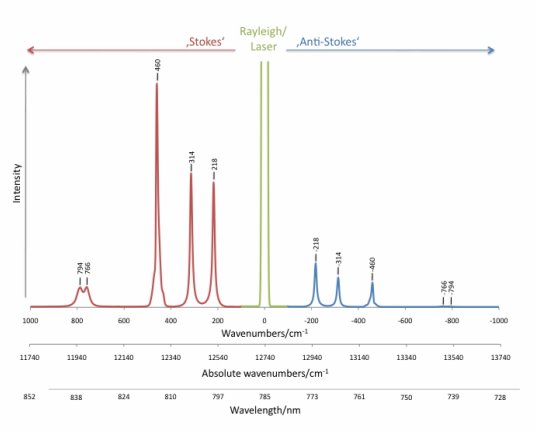
When a photon interacts with a molecule, the energy from the incident radiation is transferred to the molecule and distorts the distribution of the electron cloud. Electrons are excited to a state called the “virtual state,” where the lifetime is short. Then, the electrons drop back to the ground state and radiate light with the same frequency as the incident light and with random direction. This elastic process is called Rayleigh scattering, with the characteristic that the frequency of the scattering light is the same as that of the incident light, but its direction is random. Compared with the other type of scattering, Rayleigh scattering is the most intense scattering one can observe. In Figure 2, the green line in the middle is the Rayleigh line.
Figure 3: The different energy states of light scattering: Rayleigh scattering, Stokes effect and anti-Stokes effect.
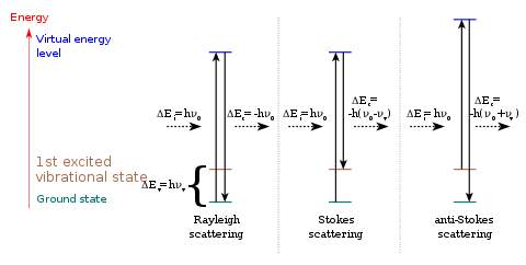
On the other hand, if the frequency of the scattering light is different from that of the incident light, this inelastic process is called Raman scattering. If the scattering frequency is higher than the incident frequency, it is the Stoke effect. If the scattering frequency is lower than the incident frequency, it is the anti-Stoke effect.
Due to thermal energy, some molecules at room temperature are initially in a higher state (such as in the first excited vibrational state, colored brown in Figure 4. After being promoted by the incident light to the “visual state” where they cannot stay for a long time, the electrons go back to the ground state and emit light with a frequency higher than that of the original light. This means that during this process, the energy in the molecule transfers to the scattering light.
The opposite with Stoke effect is the anti-Stoke effect. A molecule starts from the ground state and ends in a higher state. During this interaction, energy flows from the light to the molecule, which causes the frequency of the scattering light to be lower than that of its incident light.
The energy difference between the incident light and the scattering light is equal to the vibrational energy of the molecule. So by measuring this frequency shift, one knows the vibrational frequency of a molecule. This is the basic theory behind Raman spectroscopy. Since different chemical bonds in a molecule correspond to a variety of frequency shifts, by assigning and identifying different peaks from the Raman spectrum of an unknown molecule, one can deduce the structure and the chemical group of this molecule and categorize it.
From the thermal statistics perspective, the number of particles at different energy states of a molecule at room temperature should correspond with the Maxwell-Boltzmann distribution. The rate of the excited state and the ground state is shown below:
NnNm=gngmexp[-(En-Em)kT]
(1.1)
In equation 1.1,
Nnis the number of molecules on the excited vibrational energy level,
Nmis the number of molecules on the ground vibrational energy level, g is the degeneracy of levels n and m,
En-Emrepresents the energy difference between n and m, and k is Boltzmann’s constant.
At normal temperature, the number of molecules in the ground state is much more than in the excited state. Thus, the peak of Stoke scattering in the spectrum is higher than that of anti-Stoke scattering. Therefore, spectroscopists usually choose the frequency shift to the Stoke line to create the Raman spectrum. In Figure 2, the x-axis represents the frequency shift from incident frequency, with wavenumber cm-1 as a unit. The y-axis shows the intensity of the scattering rate. The frequency region from 500 to 1640 cm-1 is usually referred to as the fingerprint region; thus most bonds for organic material show their characteristic frequency lines in this region.
A molecule is made up of numbers of atoms forming chemical bonds. These chemical bonds may result from the electrostatic force of attraction between atoms with opposite charges or through the sharing of electrons, as in covalent bonds. If one looks into an atom, a nucleus is surrounded by an electron cloud. These electrons form the different vibrational and rotational states of the molecule.
Figure 4: The Morse potential (blue) curve and the harmonic oscillator potential (green) curve.
A
B
Figure 4 shows a sketch of a typical electronic state of a diatomic molecule. (A diatomic molecule is a molecule that only has two atoms—of the same or different molecule elements. The most common diatomic molecules are hydrogen [H2] and oxygen [O2], which are said to be homonuclear. Otherwise, if a diatomic molecule consists of two different atoms, such as carbon monoxide [CO] or nitric oxide [NO], the molecule is said to be heteronuclear [6]. The blue line of the plot, called a Morse curve, provides an institutional view of the state of the molecule. The y-axis represents the potential energy of the molecule system, and the x-axis is the separated distance between two nucleuses. The blue line represents the electronic state. When the distance between two nuclei increases, each atom is essentially free, so the system energy approaches a fixed value. As the distance decreases, two atoms attract each other and the repulsive forces increase at a rate much slower than the decreased rate of attraction. At some point, where the attraction and the repulsion reach a balance, the system energy reaches its lowest point. If these atoms keep getting closer and closer, the system energy rises steeply, while the nucleus-nucleus repulsion starts to increase rapidly over the course of the attraction. The point where the repulsion force equals the attraction is the position where the molecule system forms a chemical bond. However, not every energy state in the curve is possible for the system to stay. Based on the quantum mechanics, as the nuclei constantly oscillate around the equilibrium position between the “potential walls” of Morse potential, the energy of this vibration is quantized and described by a series of vibrational wavefunctions with their quantum numbers (v = 0, 1, 2, …). And among this vibrational state, the ground state (v = 0) is the lowest possible energy a molecule can have. At room temperature, the majority of molecules are in the lowest-energy vibrational state, but not all of them; there are still a small number of molecules that occupy the higher vibrational state. In statistics, the probability distribution of the molecules in each state can be calculated by the Maxwell-Boltzmann function.
Since the vibrational energy at the bottom of the molecule resembles that of the harmonic oscillator, one can treat the chemical bonds approximately as springs connecting nuclei obeying Hooke’s Law. The top of Figure 4 shows a model of this approach. Each ball, labeled A or B, is linked by a spring. With this approach, by applying Hooke’s Law, the relationship of the vibrations between frequencies, the mass of vibrational atoms and the force constant can be found for a diatomic molecule:
ω=12πcKμ
(1.2)
In equation 1.2, c is the velocity of light,
vis the oscillating frequency of the system, K is the force constant of the bond between atom A and B, and
μis the reduced mass of atoms A and B, given by equation 1.3:
μ=MAMBMA+MB
(1.3)
Here,
MA,
MBrepresents the mass of atoms A and B.
In such a model, the energy of each state can be represented by the following equation:
Eυ=h2π(υ+12)ω
(1.4)
According to the equation 1.4, υ = 0 1 2 …, and the vibrational energy of the molecule system can be quantized. From equations 1.1 and 1.2, one can see that the lighter the atoms, the higher the frequency. Thus, a C-H bond vibration’s frequency around 9
×108 Hz is higher than that of a C-I vibration at 1.5
×108Hz (
μH>
μI). On the other hand, the force constant can be treated as the strength of the spring (chemical bond). The stronger the bond, the higher the frequency.
This approximation provides visualization for a vibrational energy state, but one should be aware that this approximation is not entirely the same as in a real diatomic molecule’s energy state.
In equation 1.4, by calculating the energy difference between
υand
υ+1, the gap between energy levels of the harmonic oscillator is evenly spaced. However, the real bond subject to the Morse curve–quantized energy state is lower than the one of the harmonic oscillator, and the space for each energy state becomes smaller as the frequency (ω) increases.
 Amino acids are the building blocks of proteins. An amino acid is a small molecule that contains an amino group (-NH2), a carboxyl group (-COOH), a side chain (side group), and a hydrogen atom. All these groups connect to a single carbon atom at the center of the molecule, as shown in Figure 5. There are 20 different kinds of amino acids on earth. Each amino acid has a special side group that shows different chemical properties and has special peak patterns in the Raman spectrum. For example, the simplest amino acid, glycine, whose side group is a hydrogen atom, shows strong-intensity bands located at 894 cm-1 and 1,327 cm-1 in a solid state. These bands can be considered the fingerprint pattern of glycine.
The Hartree-Fock (HF) method is an approximation based on the hope that we can approximately describe an interacting fermion system in terms of an effective single-particle problem. The HF theory was developed to solve the electronic Schrodinger equation that results from the time-dependent Schrodinger equation after including the Born-Oppenheimer approximation. In atomic units, with r defining electron position and R defining nuclear degrees of freedom, the electronic Schrodinger equation is
-12∑i∇i2-∑A,iZArAi+∑A>BZAZBRAB+∑i>j1rijѰr;R=EelѰr;R
(1.5)
In order to make equation 1.5 clearly, we simplify it.
We define a one-electron operator
has follows,
hi=-12∇i2-∑AZAriA
(1.6)
and a two-electron operator
vi,jas follows:
vi,j=1rij
(1.7)
Now, we can write the electronic Hamiltonian and the electronic Schrodinger equation much more simply, as:
Hel=∑ih(i)+∑i<jvi,j.
(1.8)
VNN,which represents the inter-nucleus potential energy, is missing above. Since it is just a constant for the fixed set of nuclear coordinates, we ignore it. So our electronic Schrodinger equation becomes:
HelѰr;R=EelѰr;R
(1.9)
The essential idea of the HF theory is based on the following. We have already known the way to solve the electronic Schrodinger equation for hydrogen, which has only one electron. If we add one more electron to the hydrogen system, and assume that each electron don’t interact with the other, we can make an assumption that the total electronic wavefunction
Ѱr1;r2become
Ѱr1Ѱr2.
So if we expand the two-electron system to a multi-electron system, our wavefunction is represented as:
ѰHPx1,x2,…,xN=χ1×1χ2×2…χ1xN.
(1.10)
χNxN
is defined as the spin orbital of the number N electron.
But apparently, this assumption fails to satisfy the antisymmetry principle. Antisymmetry principle states that if any set of space-spin coordinates of a wavefunction describing fermions interchange, this wavefunction should be antisymmetric. Therefore, we need to introduce Slater Determinants.
A Slater Determinant is a determinant of spin orbitals as shown below:
Ѱ=1N!χ1×1⋯χNx1⋮⋱⋮χ1xN⋯χNxN
(1.11)
This form satisfies the antisymmetry requirement for any orbitals. The Slater Dterminant is a more sophisticated statement of the Pauli Exclusion Principle.
Now that we have a form for the wavefunction and a simplified notation for the Hamiltonian, we can start to calculate the molecular orbitals.
First, the energy of this N-body system is given by the usual quantum mechanical expression:
Eel=Ѱ|Hel|Ѱ
(1.12)
For symmetric energy expressions, we can use the variational theorem. Variational theorem states that the energy is always larger to the true energy. Therefore, we can have better approximate wavefunctions
Ѱwithin the functional space by changing their parameters until we minimize the energy. Hence, the correct molecular orbitals are those that minimize the electronic energy Eel.The molecular orbitals can be expanded as a linear combination of a set of given basis functions and named the “atomic orbital” basis set.
Now, we rewrite the HF energy Eel in terms of integrals of the one- and two-electron operators:
EHF=∑ii|h|j+12∑ijiijj-[ij|ji]
(1.13)
where the first term is the one-electron integral:
i|h|j=∫dx1χi*x1h(r1)χj(x1)
(1.14)
and a two-electron integral is
ijji=∫dx1dx2χi*x1χj(x1)1r12χk*x2χl(x2)
(1.15)
In the next step, we minimize the HF energy expression with respect to changes in the orbitals
χi→χi+δχi. We set
δEHFχi=0to try to get the minimum energy value with respect to a small change to
χi, and working through some algebra, we eventually arrive at the HF equations defining the orbitals:
hx1χix1+∑j≠i∫dx2χjx22r12-1χix1-∑j≠i∫dx2χj*(x2)χi(x2)r12-1χjx1=ϵiχix1
(1.16)
where
ϵiis the energy eigenvalue associated with orbital
χi.
The HF equations can be solved numerically. From this equation, we can see that the solutions
ϵiactually depend on the orbitals; therefore, we cannot solve this equation directly. Instead, we have to guess some initial orbitals and iterative refine our guesses through the HF method until it reaches the setting criterion. For this reason, HF is called a self-consistent-field (SCF) approach.
A basis set in the computational simulation is a set of functions (also called “basis functions”) that consists in linear combinations to represent molecular orbitals. These functions can be theoretically any types, but most of them are typically atomic orbitals centered on atoms but can be any function.
By using molecular orbitals, we can construct wavefunctions for the electronic states to describe the electronic states of molecules.For mathematical representation, a function for a molecular orbital is constructed as below:
Ѱi=∑jcijφj
(1.17)
Ѱi
is a linear combination of other functions, and
φjprovides the basis for representing the molecular orbital.
The ultimate goal for scientists is to create a description of electrons in molecules that enables chemists and other scientists to develop a deeper understanding of chemical bonding and reactivity in order to calculate the properties of a multi-body system.
In present-day computational chemistry, quantum chemical calculations are usually performed using a finite set of basis functions. For a molecular simulation, parameters of the basis functions and the coefficients in a linear combination can be optimized in terms of the Variational Theorem to produce a SCF for the electrons. According to the Variational Theorem, the calculated energy is always higher than true energy. Therefore, the ground-state energy calculated is minimized is called optimization with respect to the changing in the parameters and coefficients defining the function. As a result, if we can find the coefficients with the lowest energy of the wave function, we can get the closest value to the ground-state energy.
Depending on the different basis functions used to combine the wavefunctions, there are serval types of basis sets. I provide three basis sets as an example below.
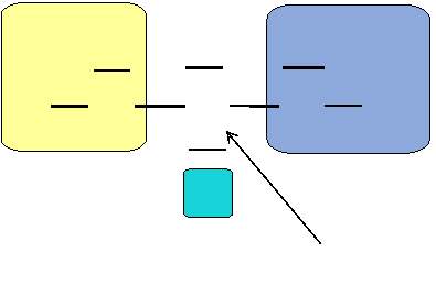
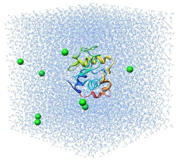
The first type is called a Gaussian Orbital, which consists of a set of Gaussian functions representing the atomic orbital of a molecule. The computation of the integrals is greatly simplified by using Gaussian-type orbitals (GTOs) for the basis functions.
A Gaussian basis function has the form shown in Equation 1.17.
Gnlmr,θ,ψ=Nnrn-1e-αr2Ylm(θ,ψ)
(1.18)
Note that in all the basis sets, only the radial part of the orbital changes, and the spherical harmonic functions are used in all of them to describe the angular part of the orbital.
Figure 6: Fixed linear combination of Gaussian functions to construct GTO basis.
As shown in Figure 6, GTO basis sets are constructed from fixed linear combinations of Gaussian functions. The abbreviations of Gaussian basis sets are identified in a way like N-MPG*. N indicates the number of Gaussian primitives used for each inner-shell orbital. M denotes the number of primitives that form the large zeta function (for the inner valence region). P indicates the number that forms the small zeta function (for the outer valence region). G represents the set is Gaussian. An asterisk at the end means that it included a single set of Gaussian 3d polarization functions.
For example, 3-21G means each inner shell is a linear combination of six primitives, and each valence shell is constructed with two sizes of basis function (Two GTOs for contracted valence orbitals; One GTO for extended valence orbitals). Accordingly, there are total of nine functions in a 3-21G basis set.
The second type of basis set is aug-cc-pvdz, also called ACCD. These are Dunning’s correlation-consistent basis sets, introduced by T.H. Dunning [7, 8]. They have had redundant functions removed and have been rotated in order to increase computational efficiency.
Polarized basis sets (POLs) were developed by Sadlej et al. [9, 10]. They were designed to improve the calculation of first- and second-order molecular properties. They consist of a standard double-zeta GTO basis with a set of extra functions derived from derivatives of the outer valence function of the original set.
2.6.1 GAMESS
Quantum chemistry computer codes are used in computational chemistry to implement the methods of Quantum Chemistry. Most of these programs include the HF method and some post-HF methods. Some of them might use density functional theory (DFT), molecular mechanics (MD), or semi-empirical quantum chemistry methods. The programs include both open-source and commercial software. Most of them are large, often containing several separate programs, and have been developed over many years.
The open-source softwareGAMESS [11, 12] is famous for general ab initio Quantum Chemistry computation. Briefly, GAMESS can compute SCF wavefunctions from RHF, ROHF, UHF, GVB, and MCSCF. Correlation corrections to these SCF wavefunctions include second-order perturbation theory, configuration interaction, and coupled-cluster approaches, in addition to the DFT approximation. There are also some procedures can compute excited states such as CI, EOM, or TD-DFT. During the automatic geometry optimization, transition state searches, or the reaction path following, the nuclear gradients are available. The prediction of vibrational frequencies of IR or Raman intensity can perform by the computation of Hessian energy. Numerous relativistic computations including infinite-order two-component scalar relativity corrections, with various spin-orbit coupling options, are available. The large systems can be calculated by the Fragment Molecular Orbital Method which use of many of these sophisticated treatments.
A variety of molecular properties, such as simple dipole moments and frequency-dependent hyperpolarizabilities may be computed. The entire periodic table can be considered, because of many basis sets are stored internally, along with effective core potentials or model core potentials.
By using GAMESS for calculating the polarizabilities of a molecule, we can perdict its Raman spectrum.
2.6.2 GAUSSIAN
The other powerful quantum computational software is called GAUSSIAN. Right now, the latest version of GAUSSIAN is Gaussian 16. As the most widespread commercial quantum computational software, Gaussian 16 have a wide-ranging suite of the most advanced modeling capabilities. It can be used to investigate real-world chemical problems in all of their complexity, even on modest computer hardware. Gaussian 16 predicts the energies, molecular structures, vibrational frequencies, and molecular properties of compounds and reactions in a wide variety of chemical environments by starting from the fundamental laws of quantum mechanics. Any stable species and compounds that are difficult or impossible to observe experimentally process whether due to their nature (e.g., toxicity, combustibility, or radioactivity) or the inherently fleeting nature (e.g., short-lived intermediates and transition structures), Gaussian 16 can be applied. Besides the functions mentioned above, Gaussian 16 can predict a variety of spectra in both the gas phase and in solution, including IR and Raman, and spin-spin coupling constants, and resonance Raman. It can also perform an anharmonic analysis for IR, Raman, VCD, and ROA spectra.
2.6.3 GROMACS
The last computational simulation software I want to introduce mainly performs molecular dynamics. It is called GROningen MAchine for Chemical Simulations (GROMACS), and it is a multipurpose package used to perform molecular dynamics. Molecular dynamics is a model to simulate the motion for systems with hundreds to millions of particles by utilizing the Newtonian equations. It is primarily designed for biochemical molecules like nucleic acids, lipids, and proteins that have many complicated chemical bonded interactions. However, since GROMACS is extremely fast at calculating non-bonded interactions (which usually dominate simulations), many scientists also use it for research on non-biological systems, e.g. polymers. GROMACS also supports all the usual algorithms one expects from a modern molecular dynamics implementation. Its code can be run in parallel computation, using either the standard MPI communication protocol, or via “Thread MPI” library for single-node workstations. The software includes a fully automated topology builder which can build the structure of proteins and even multimeric structures. The building blocks are available for the 20 standard and some modified amino acid residues, the four nucleotide and four deoxynucleotide residues, several sugars and lipids, and some special groups and several small molecules.
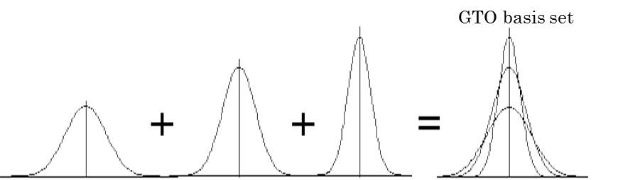
In Figure 7 below, a lysozyme in water’s molecular dynamics is simulated by MD method using GROMACS. The molecule in green and yellow at the center of the box is the lysozyme molecule, and the small blue triangles represent the water molecules. This process simulates the evolution of a lysozyme molecule interacting with water molecules over the duration of 1 ns.
Figure 7: Illustration of a simulation of lysozyme-water system
Due to the fact that simulation of biological molecules involved enormous data, need to consume significant large computational sources. The single personal computer cannot provide enormous computational sources. In order to run the molecular simulation, we need to found another powerful platform to support it. The HPC cluster is a kind of computer which can provide us powerful computational abilities. It consists of hundreds to tens of thousands multi-core processors. It allows scientists and engineers to solve complex science, engineering, and business problems using code that requires high-bandwidth networking and very high computing capabilities. A HPC cluster consists of many cores and processors, large amounts of memory, high-speed interprocessor communication networking, and large data stores—all shared across many rack-mounted servers. Due to these characteristics, a HPC cluster is usually used to run computationally intense tasks such as the simulation of physical phenomena for studying climate change and galaxy formation.
Figure 8 shows the architecture of a HPC cluster with 32 nodes. As we can see, there are several parts. First, clients can remotely log in to the cluster through the network switch. Once they log in to the cluster, they can send a task to the head node, whose main function is to distribute the task to several jobs and ask the job node to do the computation. During the computation, data are stored in the storage node, and once the task is done, the result is sent to the head node; the client can download the results from the head node. This is the processes for utilizing the HPC cluster.
Figure 8: Basic components of a HPC cluster.

Cite This Work
To export a reference to this article please select a referencing stye below:
Related Services
View all


Related Content
All TagsContent relating to: "Organic Chemistry"
Organic chemistry is a branch of chemistry that studies the chemical composition, properties, and reactions of organic compounds that contain carbon.
Related Articles

DMCA / Removal Request
If you are the original writer of this dissertation and no longer wish to have your work published on the UKDiss.com website then please: