Geo-Spatial Data Analysis for Pattern Prediction
Info: 18439 words (74 pages) Dissertation
Published: 11th Dec 2019
Tagged: GeographyTechnology
CHAPTER 1
INTRODUCTION
The most essential feature in this competitive world is data, which helps to reach conclusion about certain factors that remain unknown. This project makes use of the same to analyze the patterns. Geo spatial Data refers to the geographical data pertaining to the region, here such data is stored into data analysis platform using trees. Thus, the analyzed data provides an individual the ability to discover the patterns from the data, which is the probabilistic and effective method. The data from the real world is transformed into raster and vector format where it elevates the entities as contours and lines. The form of the spatial data which we utilized is the shapefiles, where we visualized the real-world data in form of a map.
Geospatial investigation, or simply spatial examination, is a way to deal with applying factual investigation and other explanatory procedures to information which has a geological or spatial perspective. Such examination would regularly utilize programming equipped for rendering maps handling spatial information, and applying analytical techniques to earthbound or geographic datasets, including the utilization of geographic data frameworks and geomatics. Vector-based GIS is normally identified with operations, for example, map overlay (joining at least two maps or guide layers as indicated by predefined rules), basic buffering (distinguishing areas of a map inside a predetermined separation of at least one feature, such as, towns, streets and rivers) and comparative fundamental operations. This reflects (and is reflected in) the utilization of the term spatial analysis inside the Open Geospatial Consortium (OGC) “simple feature specifications”.
For raster-based GIS, broadly utilized as a part of the ecological sciences and remote detecting, this commonly implies a scope of activities connected to the grid cells of at least one maps (or pictures) regularly including filtering as well as mathematical operations (outline). These methods include preparing at least one raster layers for every simple rule bringing about new map layer, for instance replacing every cell value with some combination of its neighbors’ qualities, or figuring the total or contrast of particular property estimations for every grid cell in two coordinating raster datasets. Illustrative insights, for example, cell tallies, means, variances, maxima, minima, combined qualities, frequencies and a few different measures and separation calculations are additionally frequently incorporated into this nonspecific term spatial examination. Spatial investigation incorporates a vast assortment of measurable methods (unmistakable, exploratory, and logical measurements) that apply to information that differ spatially and which can fluctuate after some time. Some more progressed measurable procedures incorporate Getis-ord Gi* or Anselin Local Moran’s I which are utilized to decide clustering patterns of spatially referenced information.
Traditionally geospatial figuring has been performed basically on (PCs) or servers. Because of the expanding capacities of cell phones, be that as it may, geospatial processing in cell phones is a quickly developing pattern. The compact way of these gadgets, and also the nearness of valuable sensors, for example, Global Navigation Satellite System (GNSS) collectors and barometric weight sensors, make them helpful for catching and preparing geospatial data in the field. Notwithstanding the neighborhood handling of geospatial data on cell phones, another developing pattern is cloud-based geospatial processing. In this design, information can be gathered in the field utilizing cell phones and after that transmitted to cloud-based servers for further handling and extreme stockpiling. In a comparable way, geospatial data can be made accessible to associated cell phones by means of the cloud, enabling access to immeasurable databases of geospatial data anyplace where a remote information association is accessible.
- SCOPE AND PURPOSE OF THE SYSTEM
This project is built on the concept of Geo-spatial data obtained from the maps of a city. The data must be stored in order to analyze; hence we use R-trees to store the data as contours and points. We use R platform for analyzing the Geo-spatial data. The data is imported into the Rstudio software and we arrange the data. Based on the data thus imported we clean the data and use the data mining algorithms. We choose the algorithm based on the optimized result it provides, then we predict the unknown value based on the known factors. We then visualize the predicted pattern on the maps based on the result generated from the analysis. The visualization on the map provides a clear picture of the alternatives available and gives real time proven solutions, which are dependent on the data. It helps people to arrive to a decision based on the patterns generated.
1.2 EXISTING SYSTEM
The transition of the technology from the stone age till this technological era is mainly destined in the search of innovative things. People are interested in making the life easier by accommodating it with data and the devices. To mention this, consider spatial data and its applications that have been wide spread, google maps is the primary application that uses geospatial data analysis in analysing the traffic in a particular region. But there needs an improvement for every system as the time changes.
1.3 PROPOSED SYSTEM
The primary objective of the system is to enhance the spatial data visualization with help of trees. This can be achieved by utilizing the packages in both R platform and Python by interfacing them. The spatial data of a region is aggregated from the spatial database which is in the format of shapefile, and inserted into the tree with the help of boundary box. To further utilize the analysis features in R statistical software we interface these software’s using rPython-win package. Here the analysis and the plotting of the spatial data is visualized in the form of map on the region forecasted in the shapefile.
CHAPTER 2
LITERATURE SURVEY
LITERATURE SURVEY
2.1 SPATIAL DATA:
Data is the primary source of the information that helps and guides the people to solve certain factors that remain unknown and bizarre. Generally, sources of data might vary depending on the context where the data is utilized. In its purest form, a database is simply an organized collection of information. A database management system (DBMS) is an interactive suite of software that can interact with a database. People often use the word “database” as a catch-all term referring to both the DBMS and the underlying data structure. Databases typically contain alpha-numeric data and in some cases binary large objects, or blobs, which can store binary data, such as images. Most databases also allow a relational database structure in which entries in normalized tables can be referenced to each other to create many-to-one and one-to-many relationships among data.
Spatial databases use specialized software to extend a traditional relational DBMS or RDMS to store and query data defined in two-dimensional or three-dimensional space. Some systems also account for a series of data over time. In a spatial database, attributes about geographic features are stored and queried as traditional relational database structures. The spatial extensions allow you to query geometries using Structured Query Language (SQL) in a similar way to traditional database queries. Spatial queries and attribute queries can also be combined to select results based on both location and attributes.
Spatial indexing is a process that organizes geospatial vector data for faster retrieval. It is a way of prefiltering the data for common queries or rendering. Indexing is commonly used in large databases to speed up returns to queries. Spatial data is no different. Even a moderately-sized geodatabase can contain millions of points or objects. If you perform a spatial query, every point in the database must be considered by the system to include it or eliminate it in the results. Spatial indexing groups data in ways that allow large portions of the data set to be eliminated from consideration by doing computationally simpler checks before going into detailed and slower analysis of the remaining items.
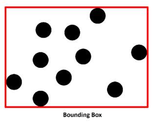
Fig 2.1.1 Format of the bounding box surrounding spatial points
Each format contains its own challenges for access and processing. When you perform analysis on data, usually you have to do some form of preprocessing first. You might clip a satellite image of a large area down to just your area of interest. Or you might reduce the number of points in a collection to just the ones meeting certain criteria in your data model. The state data set included just the state of Colorado rather than all 50 states. And the city dataset included only three sample cities, demonstrating three levels of population along with different relative locations.
Geospatial analysts benefited greatly from this market shift in several ways. First, data providers began distributing data in a common projection called Mercator. The Mercator projection is a nautical navigation projection introduced over 400 years. All projections have practical benefits as well as distortions. The distortion in the Mercator projection is size. In a global view, Greenland appears bigger than the continent of South America. But, like every projection, it also has a benefit. Mercator preserves angles. Predictable angles allowed medieval navigators to draw straight bearing lines when plotting a course across oceans. Google Maps didn’t launch with Mercator. However, it quickly became clear that roads in high and low latitudes met at odd angles on the map instead of the 90 degrees. Because the primary purpose of Google Maps was street-level driving directions, Google sacrificed the global view accuracy for far better relative accuracy among streets when viewing a single city. Competing mapping systems followed suit. Google also standardized on the WGS 84 datum. This datum defines a specific spherical model of the Earth called a geoid. This model defines the normal sea level. What is significant about this choice by Google is that the Global Positioning System (GPS) also uses this datum. Therefore, most GPS units default to this datum as well, making Google Maps easily compatible with raw GIS data. It should be noted that Google tweaked the standard Mercator projection slightly for its use; however, this variation is almost imperceptible.
2.2 SHAPEFILES:
The most ubiquitous geospatial format is the Esri shapefile. Geospatial software company Esri released the shapefile format specification as an open format in 1998 (http://www.esri.com/library/whitepapers/pdfs/shapefile.pdf). Esri developed it as a format for their ArcView software, designed as a lower-end GIS option to complement their high-end professional package, ArcIinfo, formerly called Arc/INFO. But the open specification, efficiency, and simplicity of the format turned it into an unofficial GIS standard, still extremely popular over 15 years later. Virtually every piece of software labeled as geospatial software supports shapefiles because the shapefile format is so common. For this reason, you can get by as an analyst being intimately familiar with shapefiles and mostly ignoring other formats. You can convert almost any other format to shapefiles through the source format’s native software or a third-party converter like the OGR library.
One of the most striking features of a shapefile is that the format consists of multiple files. At a minimum, there are three and there can even be as many as 15 different files! The following table describes the file formats. The .shp, .shx, and .dbf files are required for a valid shapefile.
Another important feature of shapefiles is that the records are not numbered. Records include the geometry, the .shx index record, and the .dbf record. These records are stored in a fixed order. When you examine shapefile, records using software, they appear to be numbered. But people are often confused when they delete a shapefile record, save the file, and reopen it; the number of the record deleted still appears. The reason is the
shapefile records are numbered dynamically upon loading, but not saved. So, if you delete record number 23 and save the shapefile, record number 24 will become 23 next time you read the shapefile. Many people expect to open the shapefile and see the records jump from 22 to 24. The only way to track shapefile records that way is to create a new attribute called ID or similar in the .dbf file and assign each record a permanent, unique identifier.
The shapefile format that was presented with ArcGIS version 2 in the early 1990s, do not have the ability to store the information regarding topology. It is a digital vector storage format used for associating the attributes information and to store the geometrical locations. With this now, there is a possibility for reading and writing the terrestrial datasets with extensive variety of software using this shapefile format. Because of the capability to store the undeveloped geometrical data types of points, lines, contour polygons etc., and these shapes along with various attributes of data are able to generate unlimited number of geographic data representations to provide accurate and powerful computations.
Since the shapefile format is a collection of common filename prefix files that are stored in the same directory, it is quite confusing because of its name, “shapefile”. The extensions of filenames such as .shp, .shx, and .dbf are the three mandatory files to have in the shapefile. The additional supporting files are also required along with the .shp file which is very specific to the actual shapefile to sum up as complete. Though files with long names are accepted by present-day software applications, the software of Legacy GIS expects the names of files to be restricted to eight characters in order to match the DOS 8.3 convention of filenames.
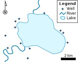
Fig. 2.2.1 Example of a shape file
2.3 DATA VISUALIZATION:
Data visualisation is viewed by many practices and disciplines as a present-day counterpart of visual communication. It involves the study and creation of the visual representation of data in the context of “information or data that has been preoccupied in some schematic form, including variables or attributes for the units of information”. The main intention of data visualization techniques is to interact with information and then clearly and effectively explain with the help of visual plots, graphs or information in graphical representations. To visibly convey a significant message, dots, lines, or bars are used to encode the numerical data. Effective visualization helps users analyse and reason about data and evidence and also makes complex data more understandable, accessible and usable. Users may have analytical or analysing tasks, such as making contrasts and comparisons or understanding connections, and the principle of design of the graphics (i.e., showing contrasts or showing origins) follows the task. To come up with a specific measurement, tables are used by the users for general purpose, while to show the specific relationships or patterns in one or more data variables, different types of charts are used.
Data visualization is termed as both a science and an art. Some view it as a descriptive statistics branch and some view as a base theory development tool. The extensive growths of the data generated by both the internet and by the remote sensors are mentioned as both Big Data and Internet of Things (IOT) correspondingly. Processing, analysing and communicating this data present ethical and analytical challenges for data visualization. Data scientists help in addressing the challenges regarding data and information in the data science field. The techniques to interact with data and information by the visual objects graphics encoding corresponds to Data visualization. It doesn’t mean that data visualization needs to be boring or sophisticated to be either functional or to be more beautiful. To communicate ideas in a more effective way, both artistic form and functionality need to go conjointly, providing a deeper knowledge into a rather scarce and complex data set by connecting its key-aspects in a more perceptive way. Yet designers often fail to attain a balance between function and form, creating impressive data visualizations which fail to serve their primary purpose.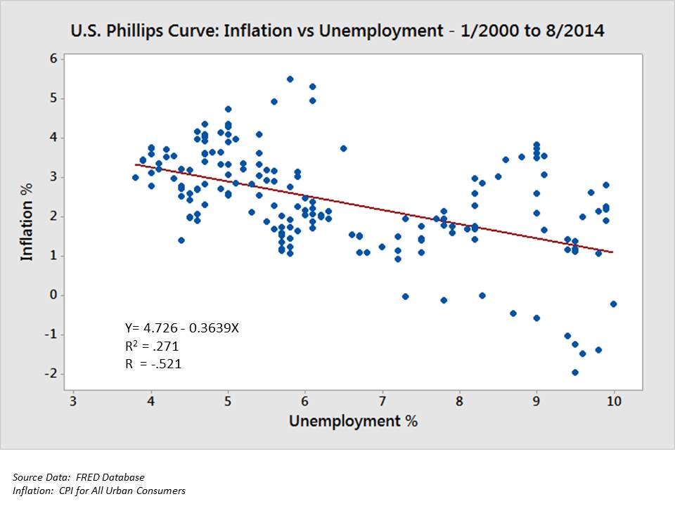
Fig. 2.3.1 Example of Data visualization technique – Scatter Plot
CHAPTER 3
SYSTEM ANALYSIS, FEASIBILTY STUDY AND REQUIREMENTS
SYSTEM ANALYSIS, FEASIBILTY STUDY AND REQUIREMENTS
3.1 SYSTEM ANALYSIS
This System Analysis is firmly identified with necessities investigation. It is likewise “an express formal request completed to help somebody distinguish a better course of action and settle on a superior choice than he/she may somehow or another have made. This progression includes separating the framework in various pieces to examine the circumstance, investigating venture objectives, separating what should be made and endeavoring to connect with clients so that unmistakable necessities can be characterized.
Performance is calculated from the output which is obtained from the application. Requirement specification has a major role in the investigation of the system. It is mostly related to the users of existing system for giving the requirement specifications as these people will be finally using the system. This is because all the requirements should be known from the starting stages therefore the whole system can be made based on those requirements. It is hard to make any corrections to the system when it has been designed and for the designing system which is not provide requirements for the user nd is of no use.
The requirement specification for a particular system is classified as:
The system must be capable to create an interface with the existing system
The system has to be accurate
The system has to be better than the existing system
The existing system is entirely depending on the user to execute all the work.
3.2 FEASIBILITY STUDY
The feasibility of the project is dissected in this stage and business proposition is advanced with an exceptionally broad arrangement for the project and some cost estimates. This is to guarantee that the proposed framework is not a weight to the organization. For possibility examination, some comprehension of the real necessities for the framework is fundamental. Three key contemplations required in the feasibility analysis are economic feasibility, technical feasibility and social feasibility.
3.3 ECONOMICAL FEASIBILITY
This review is completed to check the monetary effect that the framework will have on the association. The measure of store that the organization can fill the innovative work of the framework is restricted. The consumptions must be supported. Accordingly, the created framework too inside the financial plan and this was accomplished on the grounds that the vast majority of the advances utilized are unreservedly accessible. Just the modified items must be acquired
3.4 TECHNICAL FEASIBILITY
This review is completed to check the technical feasibility, that is, the technical requirements of the framework. Any framework created must not have much demand on the available technical resources. This will prompt levels of popularity on the available technical resources. This will lead to the high demands being set on the customer. The created framework must have an unobtrusive necessity; as just negligible or invalid changes are required for executing this framework
3.5 SOCIAL FEASIBILITY
The part of study is to check the level of acknowledgment of the framework by the client. This incorporates the way toward preparing the client to utilize the framework productively. The client must not feel undermined by the framework, rather should acknowledge it as a need. The level of acknowledgment by the clients exclusively relies on upon the techniques that are utilized to teach the client about the framework and to make him comfortable with it. His/her level of certainty must be raised so he is additionally ready to make some valuable feedback, which is invited, as he/she is the last client of the framework.
3.6 SYSTEM REQUIREMENTS
Software Requirements Specification has a major role in making a good quality software solutions. Specification is normally based on a representation procedure. Requirements are shown in a method that finally makes a successful software implementation.
Requirements can be shown in many ways. However, there are few procedures that have to followed:
- The format of Representation and data have to be connected to the problem
- Information which is in the specification has to be nested
- Diagrams and all the notational forms have to be restricted in number.
- Representations have to be revisable.
The software requirements specification is created at the perfection of the examination assignment. The capacity and execution designated to the software as a piece of framework building are refined by setting up an entire data portrayal, an itemized useful and behavioral depiction, and sign of performance requirements and outline limitations, suitable approval criteria and other information correlated to necessities.
A Software Requirements Specification (SRS) – a necessities detail for a product framework is an entire description of the conduct of a framework to be created. It incorporates an arrangement of utilization cases that depict every one of the connections the clients will have with the product. Notwithstanding use cases, the SRS additionally contains non-practical prerequisites. Non-useful necessities are requirements which force limitations on the plan or execution, (for example, performance engineering requirements, quality guidelines, or design constraints).
System requirements specification: An organized gathering of data that exemplifies the necessities of a framework. A business examiner, at times titled framework investigator, is in charge of breaking down the business needs of their customers and partners to help distinguish business issues and propose arrangements. Inside the frameworks advancement lifecycle space, the BA regularly plays out a contact work between the business side of an endeavor and the data innovation office or outside specialist organizations. Undertakings are liable to three sorts of requirements:
Business requirements depict in business terms what must be conveyed or accomplished to some benefit. Product necessities depict properties of a framework or item (which could be one of several approaches to finish an arrangement of business prerequisites.) Process necessities depict exercises performed by the creating association. For instance, prepare prerequisites could determine.
Preparatory examination looks at project attainability; the probability the framework will be useful to the association. The primary target of the feasibility study is to test the Technical, Operational and Economical feasibility for including new modules and investigating old running framework. All framework is attainable on the off chance that they are boundless assets and unending time. There are perspectives in the achievability think about bit of the preparatory examination
3.6.1 HARDWARE REQUIREMENTS
The most widely recognized set of requirements characterized by any operating system or programming application is the physical PC assets, otherwise called hardware, A hardware requirements list is regularly joined by an hardware compatibility list (HCL), particularly in the event of operating systems. A HCL records tested, compatible, and some incompatible hardware devices for a specific working framework or application. The accompanying are the hardware requirements utilized.
- 4GB /8 GB RAM
- Windows 7/8/10 64- bit
3.6.2 SOFTWARE REQUIREMENTS
Software requirements manage characterizing programming asset necessities and essentials that should be introduced on a PC to give ideal working of an application. These necessities or requirements are by and large excluded in the software installation package and should be installed separately before the software is installed.
A computer platform portrays structure, either in hardware or software, which enables software to run. Regular platforms embody a system’s architecture, programming languages or their runtime libraries and operating system.
When we consider the requirements of the framework like programming, operating system plays a major role. software may not be good with various forms of same line of working frameworks, albeit some measure of in reverse similarity is regularly kept up. For instance, most programming intended for Microsoft Windows XP does not keep running on Microsoft Windows 98, even though the opposite is not generally genuine. Likewise, programming planned utilizing more current elements of Linux Kernel v2.6 for the most part does not run or order legitimately (or by any stretch of the imagination) on Linux disseminations utilizing Kernel v2.2 or v2.4.
Programming making broad utilization of special hardware devices, similar to top of the line show connectors, needs unique API or newer device drivers.
The following are the software requirements used.
- R console
- Python
- Windows OS
- RJSONIO
CHAPTER 4
SYSTEM DESIGN
SYSTEM DESIGN
4.1 SYSTEM ARCHITECTURE
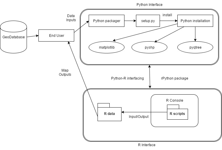
Fig 4.1.1 System Architecture
The geo spatial data is stored in the python in the form of shape files. Python packager is then being set up and then python is getting installed. It contains various packages such as pyqtree, pyshp, matplotlib. Pyqtree package helps in storing the data in the form of trees using bbox. Pyshp package helps in storing the data in the form of shapefiles, matplotlib package helps in showing the output in the form of maps. Then a interface is being established in between python and R. rpython package helps in creating an interface in between python and R. R console interprets the pattern and then show the output in the form of maps to end users.
4.2 INPUT DESIGN
The input design is the bond collaborating both information system and the end user. It constitutes the developing blueprint and strategy for data preparation and these steps are significant to put transaction data into an applicable form for processing can be produced by investigating the computer to read data from a written or printed document or it can happen by having people keying the data precisely into the system. The design of input targets on regulating the extent of input appropriate, controlling the errors, averting delay, abstaining extra stages and keeping the process uncomplicated. The input is implemented in such a manner so that it provides security and ease of use with confining the privacy.
When designing the input, that needs to be assigned the below things needs to be followed:
- What data should be given as input?
- How the data should be arranged or coded?
- The dialog to guide the operating personnel in providing input.
- Methods for preparing input validations and steps to follow when error occurs.
OBJECTIVES
- Input Design is the process of converting a user-oriented description of the input into a computer-based system. This layout is imperative to avert errors in the process of inputting data and display the legitimate direction to the authority for generating factual information from the digital system.
- It is achieved by creating user-friendly screens for the data entry to handle large volume of data. The objective of designing input is to make the process of entering the data manageable and to be withheld from errors. The data entry screen is designed in a manner such that all the data manipulation can be performed. It also provides record viewing facilities.
- When the data is entered, it will check for its validity. Data can be entered with the help of screens. Acceptable messages are provided as once required so that the user won’t be in maize of instant. Thus, the target of input style is to form Associate in guiding input layout that’s straightforward to follow.
4.3 OUTPUT DESIGN
An output with peculiarity is the one, which is expedient with the requirements of the user and manifests the information evidently. In any system, the outcome of processing is broadcasted to the end users and to various other systems through results and analysis. When we consider output design, it disposes how the knowledge is to be deranged for proximal obligation and the paper version of the output. It is the most imperative and straight forward source of knowledge to the end user. competent and astute output design upgrades the system’s liaison to help user in taking managerial decisions.
- Planning computer output ought to proceed in standardized, well thought out manner; the correct output should be developed whereas guaranteeing that every output part is intended in order that users can notice the system will use simply and effectively. once analysis style computer output, they must determine the particular output that’s required to fulfill the necessities.
- Choose methods for displaying information.
- Produce document, report, or different formats that contain data generated by the system.
- The output pattern of an information system should bring out one or more of the following objectives.
- Convey information about past activities, current status or projections of the
- Future.
- Signal important events, opportunities, problems, or warnings.
- Trigger an action.
- Confirm an action.
4.4 MODULES OF THE SYSTEM
- Python module
- R module
- Interface between statistical software’s
PYTHON:
Python has become one among the foremost standard dynamic programming languages, at the side of Perl, Ruby, and others. Such languages are typically known as scripting languages as they’ll be accustomed to write fast little programs or scripts. For data analysis and communicative, preparatory computing and data visualization, Python will necessarily derive correlation with the numerous other domain-explicit open source and commercial programming languages. Python’s enhanced library assistance (essentially pandas) has made it a potent alternative for data manipulation tasks.
Python is one of the most prominent programming languages when considered for data science and therefore its users are receiving the benefit of utilizing many pre-defined libraries that are updated and created by the Python community worldwide. Though the execution of interpreted languages, such as Python, for data processing-intensive functions is menial to lower-level programming languages, extension libraries such as Numpy and SciPy have been designed and implemented that are created upon lower layer Fortran and C applications for agile and vectorized operations on multidimensional arrays.
For machine learning programming function, the most common library imported by many data analysts is Scikit-learn, which is one of the most prominent and employable open source machine learning libraries as of today.
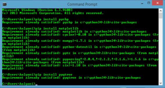
Fig. 4.4.1 Screenshot of python window (package installation)
R module:
R is a combined concatenation of software resources for data handling, computation and iconographic display. Among other things it has
- a compelling data managing and storage tools,
- an aggregation of operators for calculations on arrays, matrices,
- an extensive, comprehensible, unified assortment of transitional tools for data analysis,
- Visualization resources for data analysis and exhibit either directly at the computer or on hardcopy, and
- a well-advanced, elementary and efficient programming language (called ‘S’) which incorporates conditionals, loops, user defined recursive functions and input and output resources. (Indeed, most of the functions provided by the system are written in the S language.)
The phrase “environment” is predetermined to describe it as a completely prepared and comprehensible system, rather than a bolstering accumulation of very precise and adamant tools, as is incessant the case with other data analysis software.
R is the most prominent software for the newly implementing packages that can be utilized for the purpose of data analysis and mining. It has advanced briskly, and has been protracted by a large compilation of packages. However, most programs written in R are essentially transitory, generally written for a single piece of data analysis. The introduction which we made here is not definitely for statistics, but many people still refer to R and use it as statistics system. We prefer to think of it of an environment within which many classical and modern statistical techniques have been implemented.
Only a few of them are considered to be inbuilt with the R base environment but most of the other features are developed as packages. There are about 25 packages supplied with R (called “standard” and “recommended” packages) and many more are available through the CRAN family of Internet sites (via https://CRAN.R-project.org) and elsewhere.
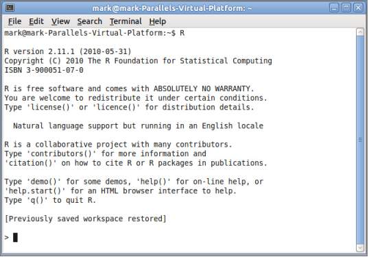
Fig. 4.4.2 A screenshot of R screen
Interface between statistical software’s (R and Python):
Statistical software’s are being used to derive the information from the unknown data and mostly for the enhanced visualization. But its unsure that only one statistical software provides all the essential features required for analysis and visualization, hence we are opting the method where we integrate different statistical software’s to receive the benefits and utilize the features of the both.
Here we consider the situation where we form the interface between Python and R, this is possible by installing packages like R tools, Dev Tools and rPython, where we need to edit the code in the configuration of rPython which points to the path of Python. Hence the files can be transferred between the platforms stimulating enhanced output.
4.5 UML CONCEPTS
The Unified Modelling Language (UML) is a standard language for writing software blue prints. The UML is a language for
- Visualizing
- Specifying
- Constructing
- Documenting the artefacts of a software intensive system.
The UML is a language which provides vocabulary and the rules for combining words in that vocabulary for the purpose of communication. A modelling language is a language whose vocabulary and the rules focus on the conceptual and physical representation of a system. Modelling yields an understanding of a system.
4.5.1 Building Blocks of the UML
The terminology of the UML comprises of three kinds of building blocks:
- Things
- Relationships
- Diagrams
Things are the abstractions that are first-class citizens in a model; relationships tie these things together; diagrams group interesting collections of things.
4.5.1.1 Things in the UML
There basically are four sorts of things within the UML:
- Structural things
- Behavioral things
- Grouping things
- Annotational things
Structural things represent the nouns of UML models. The structural things employed in the project style are:
First, a class speaks for description of a group of objects that share constant attributes, operations, relationships and linguistics.
| Window |
| Origin
Size |
| open()
close() move() display() |
Fig 4.5.1.1.1: Classes
Second, a use case may be a description of set of sequence of actions that a system performs that yields associate degree evident results of worth to explicit actor.
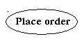
Fig 4.5.1.1.2: Use Cases
Third, a node is a physical element that exists at runtime and represents a computational resource, generally having at least some memory and often processing capability.
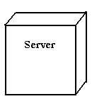
Fig 4.5.1.1.3: Nodes
Behavioral things are the dynamic parts of UML models. The behavioral thing used is:
Interaction:
An interaction serves as a behavior that includes a group of messages changed among a group of objects at intervals a selected context to accomplish a selected purpose. associate degree interaction involves variety of alternative components, as well as messages, action sequences (the behavior invoked by a message, and links (the affiliation between objects).
Fig 4.5.1.1.4: Messages
4.5.1.2 Relationships in the UML:
There basically are four forms of relationships within the UML:
- Dependency
- Association
- Generalization
- Realization
A dependency is a semantic relationship between two things in which a change to one thing may affect the semantics of the other thing (the dependent thing).
Fig 4.5.1.2.1: Dependencies
An association is a structural relationship that describes a set links, a link being a connection among objects. Aggregation is a special kind of association, representing a structural relationship between a whole and its parts.
Fig 4.5.1.2.2: Association
A generalization may be a specialization/ generalization relationship during which objects of the specialized component (the child) area unit substitutable for objects of the generalized component (the parent).
Fig 4.5.1.2.3: Generalization
A realization is a semantic relationship between classifiers, where in one classifier specifies a contract that another classifier guarantees to carry out.
Fig 4.5.1.2.4: Realization
4.5.1.3 Diagrams in the UML
Diagram is the graphical presentation of a set of elements, rendered as a connected graph of vertices (things) and arcs (relationships). A diagram may contain any combination of things and relationships. For this reason, the UML includes nine such diagrams:
(i) Class diagram:
A class diagram shows a set of classes, interfaces, and collaborations and their relationships. Class diagrams that include active classes address the static process view of a system.
(ii) Object diagram:
Object diagrams represent static snapshots of instances of the things found in class diagrams. These diagrams address the static design view or static process view of a system. An object diagram shows a set of objects and their relationships
(iii) Use case diagram:
A use case diagram shows a set of use cases and actors and their relationships. Use case diagrams address the static use case view of a system. These diagrams are especially important in organizing and modeling the behaviors of a system. Interaction Diagrams Both sequence diagrams and collaboration diagrams are kinds of interaction diagrams Interaction diagrams address the dynamic view of a system
(iv) Sequence diagram:
It is an interaction diagram that emphasizes the time-ordering of messages
(v) Communication diagram:
It is an interaction diagram that emphasizes the structural organization of the objects that send and receive messages Sequence diagrams and collaboration diagrams are isomorphic, meaning that you can take one and transform it into the other.
(vi) State Chart diagram:
A state chart diagram shows a state machine, consisting of states, transitions, events, and activities. State chart diagrams address the dynamic view of a system. They are especially important in modeling the behavior of an interface, class, or collaboration and emphasize the event-ordered behavior of an object
(vii) Activity diagram:
An activity diagram is a special kind of a state chart diagram that shows the flow from activity to activity within a system. Activity diagrams address the dynamic view of a system. They are especially important in modeling the function of a system and emphasize the flow of control among objects.
(viii) Component diagram:
A component diagram shows the organizations and dependencies among a set of components. Component diagrams address the static implementation view of a system. They are related to class diagrams in that a component typically maps to one or more classes, interfaces, or collaborations.
(ix) Deployment diagram: A deployment diagram shows the configuration of run-time processing nodes. The components that live on them Deployment diagrams address the static deployment view of an architecture.
4.5.2 UML DIAGRAMS
4.5.2.1 Use Case Diagram
The actors in the use case diagram are analyst, user, instructor, researcher, environmentalist. The use cases in the use case diagram are acquire data from database, import data, apply data mining algorithms, visualize data, association rule mining, classification, clustering, select location map, maps. The analyst will acquire the data from database. He will apply the data mining algorithms to the data. The data mining algorithms include association rule mining algorithm, classification algorithm and clustering algorithm. The user has to request for some specific location in the map. The analyst will apply the data mining algorithms and visualize the data in the form of maps to the end user.
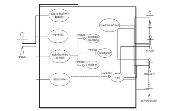 Fig 4.5.2.1.1
4.5.2.2 Class Diagram
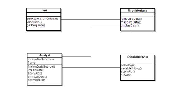
Fig 4.5.2.2.1
Each rectangle box represents a class and the upper portion of it represents class name and middle portion represents attributes of the class and the lower represents the functions performed by that class. The different classes in the class diagram are User, UserInterface, Analyst and DataMiningAlg. The methods inside the User class are selectLocationOnMap(), viewData(), getReqData(). The functions inside the UseInterface class are retrievingData(), mappingData(), displayData(). The functions inside the Analyst class are findingDataSource(), importData(), applyAlg(), analyzeData(), optimizeData(). The functions inside the DataMiningAlg are selectAlg(). variableFitting(), applyAlg(), runAlg().
4.5.2.3 Sequence Diagram
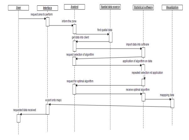
Fig 4.5.2.3.1
The Sequence diagram shows the time ordered set of instructions that has to be performed by the user. It represents sequence or flow of messages in system among various objects of the system. The rectangle boxes at top represent objects that are invoked by user and the dashed lines dropping from those boxes are life lines which shows existence of the object up to what time. The boxes on the dashed lines are events and the lines connecting them represent messages and their flow.
- Data flow diagram
A data flow diagram (DFD) is a descriptive representation of the model in which the data travels throughout the entire information system designing its mechanism traits. A DFD is generally used as a preparatory step to establish an analysis of the system by just checking the exterior points, which can later be amplified. DFDs also can be used for the visual imagination of information process (structured design).
A DFD depicts the information that which will be sent as input to the system and based on that the output derived, different phases through which the data will process, and the storage department for the data to retrieve in future. It does not show information about the timing of process or information about whether processes will operate in sequence or in parallel unlike a flowchart which also shows this information.
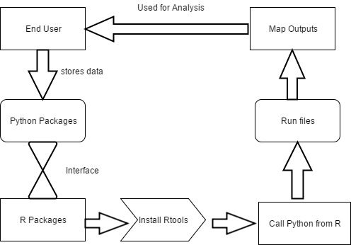
Fig 4.5.2.4.1
The end user stores the data in python in the form of shape files. Then an interface is created between python and R, using the “rPython-win” package. Then we install the R tools and devtools for the efficient working of R and Python packages. After interfacing, we call the data from python into R console and run the files in R. We use “RJSONIO” package for accepting the input data in JSON format for R statistical software. The output is represented in the form of maps and then used for analysis by the end user.
CHAPTER 5
IMPLEMENTATION AND SOFTWARE ENVIRONMENT
IMPLEMENTATION AND SOFTWARE ENVIRONMENT
5.1 PYTHON SCRIPTING LANGUAGE
Python was brought into picture by Guido Rossum van during the time of late eighties at the Institute for National Research on Mathematics and Computer Science near Netherlands. Python has been adapted and moderated from numerous different dialects, namely ABC, Algol-68-3, Unix shell, C++, MODULA, SmallTalk, and C and other scripting dialects. Python developers have made it copyrighted. Like Perl, Python source code is currently accessible under the GNU General Public License (GPL). Python is presently kept up by a center advancement group at the organization, in spite of the fact that Guido van Rossum still holds an imperative part in coordinating its encouraging.
Python is a high-level, interpreted, interactive and object-oriented scripting language. Python is intended to be highly readable. It utilizes English watchwords often whereas different dialects utilize accentuation, and it has less grammatical developments than different dialects.
Python is prepared at runtime by the interpreter. You don’t have to arrange your program before executing it. This is like PERL and PHP.
You can really sit at a Python prompt and collaborate with the interpreter straightforwardly to compose your programs.
Python bolsters Object-Oriented style or method of programming that typifies code inside objects.
Python is a language for the learner level software engineers and backings the advancement of an extensive variety of utilizations from basic content handling to WWW programs to amusements.
Python’s features include:
- It is Easy-to-learn: Python has less keywords, small structure, and a perfectly defined syntax. This makes the student to understand the language quickly.
- It is Easy-to-read: The code of the Python is more neatly defined and visible.
- It is Easy-to-maintain: Python’s source code is very easy to maintain.
- This language has A Great standard library: The large amount of the library is convertible from one platform to another.
- It has Interactive Mode: Python has buttress for an interactive mode that can allow interactive testing and debugging of snippets of code.
- It is Portable: Python can run on a large amount of hardware platforms and it has the same interface on all the platforms.
- It is Extendable: we can combine low-level modules with the Python interpreter. These modules help programmers to combine or customize for their tools to be more effective.
- Databases: Python will provide many interfaces to all higher commercial databases.
- It has graphical Programming: Language strengthens GUI applications which can be originated and transferred to numerous calls made by system, windows systems and libraries.
- It is Scalable: Python will provide a nice structure and support for huge programs when compared to shell scripting.
Aside from the previously mentioned highlights, Python has a major rundown of good components, few are recorded beneath:
- It underpins utilitarian and organized programming techniques and additionally OOP.
- It can be utilized as a scripting dialect or can be ordered to byte-code for building extensive applications.
- It gives abnormal state dynamic information sorts and backings dynamic sort checking.
- IT underpins programmed junk gathering.
- It can be effectively coordinated with C, C++, COM, ActiveX, CORBA, and Java.
5.2 R STATISTICAL SOFTWARE
R is an execution of the S programming language consolidated with lexical checking semantics enlivened by Scheme S was made by John Chambers while at Bell Labs. There are some vital contrasts, however a significant part of the code composed for S runs unaltered.
R was made by Ross Ihaka and Robert Gentleman at the University of Auckland, New Zealand, and is as of now created by the R Development Core Team, of which Chambers is a part. R is named somewhat after the primary names of the initial two R creators and halfway as a play on the name of S. The venture was considered in 1992, with an underlying rendition discharged in 1995 and a steady beta form in 2000.
R is an open source programming language and programming condition for measurable figuring and illustrations that is upheld by the R Foundation for Statistical Computing. The R language is broadly utilized among analysts and information diggers for creating factual programming and information investigation. Surveys, overviews of information excavators, and investigations of insightful writing databases demonstrate that R’s notoriety has expanded generously lately.
R is a GNU package. The source code for the R programming environment is composed basically in C, Fortran, and R.R is unreservedly accessible under the GNU General Public License, and pre-incorporated double forms are accommodated different working frameworks. While R has a charge line interface, there are a few graphical front-closes accessible.
R and its libraries execute a wide assortment of factual and graphical strategies, including straight and nonlinear displaying, established measurable tests, time-arrangement investigation, order, bunching, and others. R is effortlessly extensible through capacities and augmentations, and the R people group is noted for its dynamic commitments as far as bundles. A large portion of R’s standard capacities are composed in R itself, which makes it simple for clients to take after the algorithmic decisions made. For computationally escalated tasks, C, C++, and FORTRAN code can be connected and called at run time.
Propelled clients can compose C++, Java, .NET or Python code to control R protests specifically. R is exceedingly extensible utilizing client submitted packages for particular functions or particular zones of study. Because of its S legacy, R has more grounded question arranged programming offices than most measurable processing languages. Broadening R is likewise facilitated by its lexical perusing rules.
Another quality of R is static illustrations, which can create distribution quality diagrams, including scientific images. Dynamic and intuitive representation are accessible through extra bundles.
R has Rd, its own Latex-like documentation configuration, which is utilized to supply far reaching documentation, both on-line in many organizations and in printed copy.
R packages are combination of R functions, went along code and test information. They are put away under a registry called “library” in the R environment. As a matter, of course, R introduces an arrangement of bundles amid establishment. More packages are included later, when they are required for some particular reason. When we begin the R support, just the default packages are accessible as a matter of course. Different packages which are now introduced must be stacked unequivocally to be utilized by the R program that will utilize them.
- RPYTHON Package
This package enables the client to call Python from R. It is a characteristic augmentation of the rJython package by a similar creator. rPython is expected for running Python code from R. R programs and packages can: Pass information to Python: vectors of different sorts (legitimate, character, numeric…), records, and so on. Get information from Python. Call Python code, call Python capacities and techniques.
Version: 0.0-6
Date: 2015-11-15
Title: Package Allowing R to Call Python
Author: Carlos J. Gil Bellosta
Maintainer: Carlos J. Gil Bellosta
Description: Run Python code, make function calls, assign and retrieve variables, etc. from R.
Depends: RJSONIO (>= 0.7-3)
License: GPL-2
SystemRequirements: Python (>= 2.7) and Python headers and libraries (See the INSTALL file)
OS_type: unix
URL: http://rpython.r-forge.r-project.org/
Repository: CRAN
Date/Publication: 2015-11-15 22:27:07
5.4 PYQTREE
Pyqtree is a transparent Python quad tree that can be helpful in rendering GIS applications due to its spatial nature. It stores and rapidly recovers things from a 2×2 rectangular network territory, and develops inside and out and detail as more things are included. It is good on stages 2 and 3 of Python. It is composed in pure Python and has no conditions.
Installation:
Installation of Pyqtree is basically done by opening the terminal or command line and typing the following:
- pip install Pyqtree
Alternatively, you can easily download the “pyqtree.py” file and keep it wherever Python can import it, like the Python site-packages folder.
Usage:
You can Start writing the script by importing the module.
- import Pyqtree
firstly, you have to Setup the spatial index, have to give it the bounding box area for making track. The bounding box has a four-tuple: (xmin,ymin,xmax,ymax).
- spindex = pyqtree.Index (bbox=[0,0,100,100])
then Populate the index with which means that you want to get that retrieved at a later point, with every items geographic bbox.
Classes:
- class Index
It is the top spatial list to be made by the client. Once made it can be populated with topographically set individuals that can later be tried for crossing point with a client inputted geographic bounding box. Take note of that the record can be iterated through in a for-proclamation, which circles through all the quad cases and gives you a chance to get to their properties.
Parameters:
- bbox
It is a coordinate system bounding box for which the area of the quadtree have to keep track, it has as a 4-length sequence (xmin,ymin,xmax,ymax).
5.5 PYSHP
The Python Shapefile Library (pyshp) gives read and compose support to the Esri Shapefile organize. The Shapefile configuration is a prominent Geographic Information System vector information organize made by Esri. The Esri record depicts the shp and shx document formats. Both the Esri and XBase document arrangements are exceptionally basic in outline and memory effective which is a piece of the reason the shapefile design stays well known regardless of the various approaches to store and trade GIS information accessible today. Pyshp is perfect with Python 2.4-3.x.
A shapefile stores nontopological geometry and characteristic data for the spatial features in an informational index. The geometry for an element is put away as a shape involving a set of vector coordinates. Because shapefiles don’t have the preparing overhead of a topological information structure, they have points of interest over other information sources, for example, quicker drawing pace and editability. Shapefiles handle single elements that cover or those are noncontiguous. They also regularly require less plate space and are less demanding to peruse and write. Shapefiles can bolster point, line, and region highlights. Range elements are spoken to as closed circle, twofold digitized polygons. Characteristics are held in a dBASE arrange file. Each property record has a balanced association with the related shape record.
How Shapefiles Can Be Created:
Shapefiles can be generated by following below mentioned general methods:
- The process of Export-Shapefiles which is used to export the data present in the form a shapefile using BusinessMAP™ software, Spatial Database Engine™ (SDE™), ArcView® GIS, or PC ARC/INFO®.
- Digitize-Shapefiles can be directly made by digitizing shapes by using ArcView GIS feature creation tools.
- Programming-Using Avenue™ (ArcView GIS), MapObjects™, ARC Macro Language (AML™) (ARC/INFO), or Simple Macro Language (SML™) (PC ARC/INFO) software, you can create shapefiles within your programs.
- Writing directly to the shapefile specifications by making a program.
Before starting anything, we have to import the library.
- Then import the shapefile
Reading Shapefiles:
The procedure for reading a shapefile is to create a new “Reader” object and then pass the name of the existing shapefile. The shapefile format is the combination of three files. You have to specify the base filename of the shapefile or can specify the complete filename of any other shapefile component files.
- sf = shapefile.Reader(“shapefiles/blockgroups”)
OR
- sf = shapefile.Reader (“shapefiles/blockgroups.shp”)
OR
- sf = shapefile.Reader(“shapefiles/blockgroups.dbf”)
The library does not care about file extensions OR any of the other 5+ formats which are potentially part of a shapefile.
Reading Shapefiles from File-Like Objects:
The shapefiles can also be exported from the Python files in the form of utilizing the keyword arguments of the object to state any of the three records. This segment is adept and enables you to load shapefiles from a compress document, from a serialized object, URL, or now and again a database.
- myshp = open(“shapefiles/blockgroups.shp”, “rb”)
- mydbf = open(“shapefiles/blockgroups.dbf”, “rb”)
- r = shapefile.Reader(shp=myshp, dbf=mydbf)
Reading Geometry:
A shapefile’s geometry is a huge combination of points or shapes which are actually from vertices and implied arcs which represents physical locations. All these types of shapefiles only contain points. The metadata about these points define how they are used by software.
There is a collection of the shapefile’s geometry by calling the shapes () method.
- shapes = sf.shapes()
This shapes method will return a collection of Shape objects which describes the geometry of each and every shape record.
- len (shapes)
we can iterate from the shapefile’s geometry by making use of the iterShapes() method.
- len (list (sf.iterShapes ()))
Each and every shape record will have the following attributes:
- for name in dir(shapes[3]):
… if not name.startswith (‘__’):
… name
‘bbox’
‘parts’
‘points’
‘shapeType’
- shapeType: this is an integer which shows the type of shapes defined by the shapefile specification.
- bbox: On the off chance that the shape sort contains various focuses this tuple portrays the lower left (x,y) organize and upper right corner facilitate making a total box around the focuses. In the event that the shapeType is a Null (shapeType == 0) then an AttributeError is raised.
- parts: Parts basically amass accumulations of focuses into shapes. On the off chance that the shape record has numerous parts this characteristic contains the file of the principal purpose of each part. In the event that there is just a single part then a rundown containing 0 is returned.
- points: The focuses property contains a rundown of tuples containing a (x,y) arrange for each point in the shape.
- To peruse a solitary shape by calling its record utilize the shape() technique. The file is the shape’s number from 0. So, to peruse the eighth shape record you would utilize its list which is 7.
- s = sf.shape(7)
Reading Records:
A record in a shapefile contains the characteristics for each shape in the accumulation of geometry. Records are put away in the dbf document. The connection amongst geometry and properties is the establishment of all geographic data frameworks. This basic connection is suggested by the request of shapes and comparing records in the shp geometry document and the dbf quality document.
The field names of a shapefile are accessible when you read a shapefile. You can call the “fields” quality of the shapefile as a Python list. Each field is a Python list with the accompanying data:v
Field name: the name which describes the data in the column index.
Field type: the sort of information at this segment list. Sorts can be: Character, Numbers, Longs, Dates, or Memo. The “Reminder” sort has no importance inside a GIS and is a piece of the xbase spec.
Field length: the length of the information found at this section list. More seasoned GIS programming may truncate this length to 8 or 11 characters for “Character” fields.
Decimal length: the quantity of decimal spots found in “Number” fields.
To see the fields for the Reader protest above (sf) call the “fields” quality:
fields = sf.fields
You can get a list of the shapefile’s records by calling the records() method:
- records = sf.records()
Like the geometry strategies, you can emphasize through dbf records utilizing the iterRecords() strategy.
- len(list(sf.iterRecords()))
To read a solitary record call the record() strategy with the record’s list:
- rec = sf.record (3)
Reading Geometry and Records Simultaneously:
You need to look at both the geometry and the properties for a record in the meantime. The shapeRecord() and shapeRecords() strategy let you do only that.
Calling the shapeRecords() strategy will give back the geometry and characteristics for all shapes as a rundown of ShapeRecord items. Each ShapeRecord occasion has a “shape” and “record” characteristic. The shape property is a ShapeRecord question as talked about in the primary segment “Perusing Geometry”. The record trait is a rundown of field values as exhibited in the “Perusing Records” segment.shapeRecs = sf.shapeRecords ()
The shapeRecord() method reads a single shape/record pair at the specified index. To get the 4th shape record from the block groups shapefile use the third index:
Writing Shapefiles:
- w = shapefile.Writer ()
PyShp tries to be as adaptable as conceivable when composing shapefiles while keeping up some level of programmed approval to ensure you don’t coincidentally compose an invalid record.
PyShp can compose only one of the segment documents, for example, the shp or dbf record without composing the others. So notwithstanding being an entire shapefile library, it can likewise be utilized as a fundamental dbf (xbase) library. Dbf documents are a typical database arrange which is frequently helpful as an independent basic database design. What’s more, even shp records infrequently have utilizes as an independent configuration. Some online GIS frameworks utilize a client transferred shp record to determine a zone of intrigue. Numerous exactness horticulture compound field sprayers additionally utilize the shp arrange as a control petition for the sprayer framework (more often than not in mix with custom database record positions).
To make a shapefile you include geometry or potentially qualities utilizing strategies in the Writer class until you are prepared to spare the document.
Make an occasion of the Writer class to start making a shapefile:
Setting the Shape Type:
The shape sort characterizes the kind of geometry contained in the shapefile. The majority of the shapes must match the shape sort setting.
Shape sorts are spoken to by numbers in the vicinity of 0 and 31 as characterized by the shapefile particular. Note that numbering framework has a few saved numbers which have not been utilized yet hence the quantities of the current shape sorts are not successive.
Geometry and Record Balancing:
TBecause each shape must have a comparing record it is important that the quantity of records equivalents the quantity of shapes to make a substantial shapefile. To help avert incidental misalignment the PSL has an “auto adjust” highlight to ensure when you include either a shape or a record the two sides of the condition line up. This element is NOT turned on as a matter of course. To enact it set the credit autoBalance to 1 (True):
- w.autoBalance = 1
You additionally have the alternative of physically calling the adjust() technique each time you include a shape or a record to guarantee the opposite side is a la mode. When adjusting is utilized invalid shapes are made on the geometry side or a record with an estimation of “Invalid” for each field is made on the characteristic side.
The adjusting choice gives you adaptability by the way you fabricate the shapefile.
Without auto adjusting you can include geometry or records whenever. You can make the majority of the shapes and after that make the majority of the records or the other way around. You can utilize the adjust technique in the wake of making a shape or record each time and make refreshes later. In the event that you don’t utilize the adjust technique and neglect to physically adjust the geometry and properties, the shapefile will be seen as degenerate by most shapefile programming.
With auto adjusting you can include either shapes or geometry and refresh clear passages on either side as required. Regardless of the possibility that you neglect to refresh a section the shapefile will in any case be substantial and dealt with effectively by most shapefile programming.
Adding Geometry:
Geometry is included utilizing one of three techniques: “invalid”, “point”, or “poly”. The “invalid” strategy is utilized for invalid shapes, “point” is utilized for point shapes, and “poly” is utilized for everything else.
Adding a Point shape:
Point shapes are included utilizing the “point” technique. A point is indicated by a x, y, and discretionary z (rise) and m (measure) esteem.
- w = shapefile.Writer()
Adding a Poly shape:
“Poly” shapes can be either polygons or lines. Shapefile polygons must have no less than 4 focuses and the last point must be the same as the first. PyShp consequently authorizes shut polygons. A line must have no less than two focuses. On account of the likenesses between these two shape sorts they are made utilizing a solitary strategy called “poly”.
- w = shapefile.Writer()
Adding a Null shape:
Since Null shape sorts (shape sort 0) have no geometry the “invalid” technique is called with no contentions. This kind of shapefile is once in a while utilized yet it is substantial.
- w = shapefile.Writer()
- w.null()
Editing Shapefiles:
The Editor class endeavors to make changing existing shapefiles simpler by taking care of the perusing and composing points of interest in the background. This class is test, has loads of issues, and ought to be evaded for creation utilize.
- e = shapefile.Editor()
5.6 MATPLOTLIB
Matplotlib could be a Python 2-dimension plotting library that produces production quality figures in associate degree assortment of written copy teams and intelligent conditions crosswise over stages. Matplotlib will be utilised as a region of Python scripts, the Python and IPython shell, the jupyter scratch pad, internet application servers, and 4 graphical UI toolkits. Matplotlib tries to create easy things easy and exhausting things conceivable. You can create plots, histograms, control spectra, bar graphs, errorcharts, scatterplots, and so forth., with only a couple lines of code.For straightforward plotting the pyplot module gives a MATLAB-like interface, especially when consolidated with IPython. For the power client, you have full control of line styles, text style properties, tomahawks properties, and so forth., through a protest situated interface or by means of an arrangement of capacities commonplace to MATLAB clients.
In the event that Python 2.7 or 3.4 are not introduced for all clients, the Microsoft Visual C++ 2008 ( 64 bit or 32 bit for Python 2.7) or Microsoft Visual C++ 2010 ( 64 bit or 32 bit for Python 3.4) redistributable bundles should be introduced.
Matplotlib relies on upon Pillow for perusing and sparing JPEG, BMP, and TIFF picture documents. Matplotlib requires MiKTeX and GhostScript for rendering content with LaTeX. FFmpeg, avconv, mencoder, or ImageMagick are required for the liveliness module.
The accompanying backends ought to work out of the crate: agg, tkagg, ps, pdf and svg. For different backends you may need to introduce pycairo, PyQt4, PyQt5, PySide, wxPython, PyGTK, Tornado, or GhostScript.
TkAgg is most likely the best backend for intelligent use from the standard Python shell or IPython. It is empowered as the default backend for the official parallels. GTK3 is not upheld on Windows.
The Windows wheels (*.whl) on the PyPI download page don’t contain test information or case code. On the off chance that you need to attempt the numerous demos that come in the matplotlib source conveyance, download the *.tar.gz record and look in the illustrations subdirectory. To run the test suite, duplicate the libmatplotlib ests and libmpl_toolkits ests catalogs from the source circulation to sys.prefixLibsite-packagesmatplotlib and sys.prefixLibsite-packagesmpl_toolkits separately, and introduce nose, ridicule, Pillow, MiKTeX, GhostScript, ffmpeg, avconv, mencoder, ImageMagick, and Inkscape
Installing from source:
On the off chance that you are keen on adding to matplotlib improvement, running the most recent source code, or simply jump at the chance to manufacture everything yourself, it is not hard to construct matplotlib from source. Snatch the most recent tar.gz discharge record from the PyPI documents page, or in the event that you need to create matplotlib or simply require the most recent bug fixed variant, get the most recent git rendition Source introduce from git.
When you have fulfilled the prerequisites definite (fundamentally python, numpy, libpng and freetype), you can construct matplotlib:
- cd matplotlib
- python setup.py build
- python setup.py install
A setup.cfg record that runs with setup.pycan be utilized to redo the fabricate procedure. For instance, which default backend to utilize, regardless of whether a portion of the discretionary libraries that matplotlib ships with are introduced, et cetera. This document will be especially helpful to those bundling matplotlib.
On the off chance that you have introduced essentials to nonstandard places and need to illuminate matplotlib where they are, alter setupext.py and add the base dirs to the basedir lexicon passage for your sys.platform. e.g., if the header to some required library is in/a few/way/incorporate/someheader.h, put/a few/way in the basedir list for your stage.
Build requirements:
Required Dependencies:
These are external packages which you should introduce before introducing matplotlib. In the event that you are expanding on OSX, see Building on OSX. On the off chance that you are expanding on Windows, see Building on Windows. On the off chance that you are introducing conditions with a bundle director on Linux, you may need to introduce the advancement bundles (search for a “- dev” postfix) notwithstanding the libraries themselves.
- python 2.7, 3.4, 3.5 or 3.6
- numpy 1.7.1 setuptools: It provides extensions for python package installation.
- dateutil 1.1
- libpng 1.2 Pytz: used to manipulate time-zone aware datetimes.
- FreeType 2.3
- cycler 0.10.0
Building on Windows:
The Python transported from https://www.python.org is assembled with Visual Studio 2008 for variants before 3.3, Visual Studio 2010 for 3.3 and 3.4, and Visual Studio 2015 for 3.5 and 3.6. Python augmentations are prescribed to be accumulated with a similar compiler.
Since there is no authoritative Windows bundle supervisor, the strategies for building freetype, zlib, and libpng from source code are archived as a fabricate script at matplotlib-winbuild
Toolkits:
There are a few Matplotlib add-on toolboxs, including a decision of two projection and mapping tool stash basemap and cartopy, 3d plotting with mplot3d, tomahawks and hub partners in axes grid, a few larger amount plotting interfaces seaborn, holoviews, ggplot.
Citing Matplotlib:
Matplotlib is the brainchild of John Hunter (1968-2012), who, alongside its numerous benefactors, have put an unfathomable measure of time and exertion into delivering a bit of programming used by a huge number of researchers around the world.
Open source:
The Matplotlib permit depends on the Python Software Foundation (PSF) license. There is a dynamic engineer group and a considerable rundown of individuals who have made critical commitments. It is facilitated on Github.
5.7 RJSONIO
RJSONIO is a package that enables transformation to and from data in Javascript question documentation (JSON) arrange. This permits R articles to be embedded into Javascript/ECMAScript/ActionScript code and enables R software engineers to peruse and change over JSON substance to R objects. This is an other option to rjson bundle. Initially, that was too moderate for changing over huge R object sto JSON and was not extensible. Rjson’s execution is presently like this bundle, and perhaps slightly speedier in some cases.This bundle utilizes strategies and is promptly extensible by characterizing techniques for various classes, vectorized operations, and C code and callbacks to R capacities for deserializing JSON objects to R.
The two packages deliberately have a similar fundamental interface. This package (RJSONIO)has numerous additional options to permit tweaking the era and handling of JSON content. This package utilizes libjson instead of executing yet another JSON parser. The point is to suppor to other general undertakings by expanding on their work, giving input and advantage from their ongoing development.
This RJSONIO package utilizes the libjson C library fromlibjson.sourceforge.net. A rendition of that C++ code is incorporated in this package and can be utilized. Then again, one can utilize a differen t version of libjson, e.g. a later form. To do this, you introduce that rendition of libjson with:
- make SHARED=1 install
The key thing is to make this a mutual library so we can connect against it as position autonomous code (PIC).
As a matter of course, this will be introduced in/usr/nearby.
You can control this with,
- make SHARED=1 install prefix=”/my/directory”
The arrangement script will endeavor to discover libjson on your framework, looking in/usr/neighborhood. On the off chance that this is not the area you installed libjson to, you can indicate the prefix by means of the – with-prefix=/my/catalog.
E.g.
- R CMD INSTALL –configure-args=”–with-prefix=/my/directory” RJSONIO
- R CMD INSTALL –configure-args=”–with-local-libjson=yes” RJSONIO
CHAPTER 6
CODING AND TESTING
CODING AND TESTING
6.1 CODE
After the initial comment block and library import, the code reads in the shapefile using the string variables that give the location of the shapefile directory (data_dir) and the name of the shapefile without extension (shp_file_base):
“””
IMPORT THE SHAPEFILE
“””
Sf = shapefile.Reader(“E:/Major Project/spatial data sources/INDIA/IND_adm_shp/IND_adm2.shp”)
This creates a shapefile object, sf, and the next few lines do some basic inspections of that object. To check how many shapes have been imported:
print (‘number of shapes imported:’,len(sf.shapes()))
print (‘ ‘)
print (‘geometry attributes in each shape:’)
For each shape (or state), there are a number of attributes defined: bbox, parts, points and shapeType.
“””
PLOTTING
“””
“”” PLOTS A SINGLE SHAPE “””
The first thing we wanted to do after importing the shapefile was just plot a single state. So we first pull out the information for a single shape (in this case, the 5th shape):
shape_ex = sf.shape(7)
The points attribute contains a list of latitude-longitude values that define the shape (state) boundary. So, we loop over those points to create an array of longitude and latitude values that we can plot. A single point can be accessed with shape_ex.points[0] and will return a lon/lat pair, e.g. (-70.13123,40.6210). So we pull out the first and second index and put them in pre-defined numpy arrays:
x_lon = np.zeros((len(shape_ex.points),1))
y_lat = np.zeros((len(shape_ex.points),1))
for ip in range(len(shape_ex.points)):
x_lon[ip] = shape_ex.points[ip][0]
y_lat[ip] = shape_ex.points[ip][1]
And then I plot it:
plt.plot(x_lon,y_lat,’k’)
We also used the bbox attribute to set the x limits of the plot. bbox contains four elements that define a bounding box using the lower left lon/lat and upper right lon/lat. Since we are setting the axes aspect ratio equal here, we only define the x limit.
# use bbox (bounding box) to set plot limits
plt.xlim(shape_ex.bbox[0],shape_ex.bbox[2])
So all we need now is to loop over each shape (state) and plot it! Right? But it turns out that the parts attribute of each shape includes information to save us! For a single shape the parts attribute (accessed with shape.parts) contains a list of indices corresponding to the start of a new closed loop within a shape. So we modified the above code to first check if there are any closed loops (number of parts > 1) and then loop over each part, pulling out the correct index range for each segment of geometry:
“”” PLOTS ALL SHAPES AND PARTS “””
for shape in list(sf.iterShapes()):
npoints=len(shape.points) # total points
nparts = len(shape.parts) # total parts
if nparts == 1:
x_lon = np.zeros((len(shape.points),1))
y_lat = np.zeros((len(shape.points),1))
for ip in range(len(shape.points)):
x_lon[ip] = shape.points[ip][0]
y_lat[ip] = shape.points[ip][1]
plt.plot(x_lon,y_lat)
else: # loop over parts of each shape, plot separately
for ip in range(nparts): # loop over parts, plot separately
i0=shape.parts[ip]
if ip < nparts-1:
i1 = shape.parts[ip+1]-1
else:
i1 = npoints
seg=shape.points[i0:i1+1]
x_lon = np.zeros((len(seg),1))
y_lat = np.zeros((len(seg),1))
for ip in range(len(seg)):
x_lon[ip] = seg[ip][0]
y_lat[ip] = seg[ip][1]
plt.show()
Hence, the above code when executed plots in the following form as shown in fig. 6.1.1.
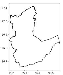
Fig. 6.1.1
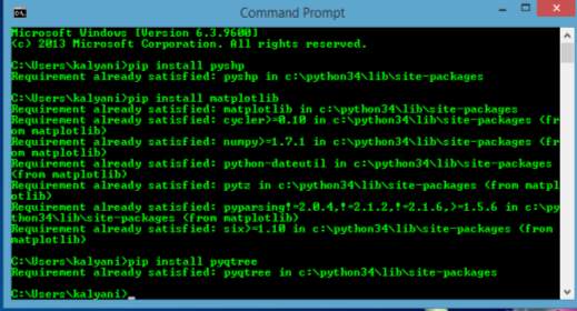
Fig. 6.1.2 Installing of packages in python
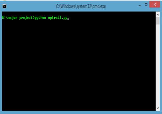
Fig. 6.1.3 Executing the python program
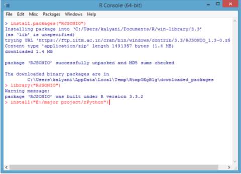
Fig. 6.1.4 Establishing the interface and running the program
6.2 SYSTEM TESTING
The main aim of testing a code is to discover or find errors. Testing is the procedure of encountering every convincing error or weakness or fault in a work product. It is a way that provides functionality check of components, assemblies, sub-assemblies and a refined product. It is the method of exerting software with the intent of assuring that the requirements of the software system are met accordingly as the user expects it to be and does not fail in an improper way. There are several types of testing for the code in which every specific testing requirement is addressed by each type of test.
6.2.1 TYPES OF TESTS
6.2.1.1 UNIT TESTING
Validating that the internal program logic is functioning properly Unit testing involves the design of test cases, and that valid outputs are produced from program inputs. All call branches and internal code flow ought to be valid. Testing of individual software package units of the appliance is finished through unit testing .it is done when the completion of a personal unit before integration. this can be a structural testing, that depends on data of its construction and is invasive. Basic checks at element level and test a selected business method, application, and/or system configuration Unit tests area unit performed. Unit tests make sure that every distinctive path of a business method performs accurately to the documented specifications and contains clearly outlined inputs and expected results.
6.2.1.2 INTEGRATION TESTING
If they really run jointly program Integration tests area unit designed to check integrated code elements to see. Testing is event driven and is additional involved with the essential outcome of screens or fields. Integration tho’ the elements were on an individual basis satisfaction tests demonstrate, as shown by with success unit testing, the mixture of elements is correct and consistent. Integration testing is specifically aimed toward exposing the issues that arise from the mixture of elements.
6.2.1.3 FUNCTIONAL TESTING
As such by the business and technical needs that Functions tested square measure accessible that done by purposeful tests offer systematic demonstrations, system documentation, and user manuals. purposeful testing is focused on the subsequent items:
Valid Input : Valid input must be authorized only of the analyzed classes.
Invalid Input : identified classes of invalid input must be repudiated.
Functions : identified functions must be exercised.
Output : identified classes of application outputs must be exercise.
Procedures : interfacing systems or procedures must be supplicated.
Organization and preparation of useful tests is concentrated on necessities, key functions, or special take a look at cases.
6.2.1.4 SYSTEM TESTING
The entire integrated package meets necessities that System testing ensures. It tests a configuration to make sure celebrated and predictable results. For a instance of system take a look at system is that the configuration orienting system integration test. System testing is predicated on method descriptions and flows, action pre-driven method links and integration points.
6.2.1.5 WHITE BOX TESTING
White Box Testing may be a testing within which the package tester has data of the inner workings, structure and language of the package, or a minimum of its purpose. its purpose. it’s accustomed take a look at areas that can’t be reached from a recording equipment level.
6.2.1.6 BLACK BOX TESTING
The package with none data of the inner workings, structure or language of the module being tested is recording equipment Testing. recording equipment tests, as most other forms of tests, should be written from a definitive supply document, like specification or necessities document, like specification or necessities document. it’s a take a look at system within which the package underneath test is treated, as a recording equipment. you cannot “see” into it. The look at provides inputs and responds to outputs while not considering however the package works.
6.3 UNIT TESTING
An element of test-driven development (TDD), a sensible methodology that takes a scrupulous approach to putting together a product by means that of continual testing and revision is Unit Testing. Test-driven development needs that developers 1st write failing unit tests. Then code is written and refactor the appliance till the take a look at passes. TDD usually ends up in an exact and foreseeable code base.
Unit testing involves solely those attributes that are necessary to the performance of the unit beneath test. This encourages developers to modify the source code without immediate concerns about how such changes might affect the functioning of other units or the program as a whole. The program can be evaluated by means of integration testing, once all of the units in a program have been found to be working in the most efficient and error-free manner possible, larger components of.
Unit testing does have steep learning curve. The development team needs to learn about how the process of testing and how and what actually unit testing means and how use automated software tools to facilitate the process on an on-going basis. The great benefit to unit testing is that the problem is detected then there is a possibility of few errors. Though eventually conflicts with something down the line and results in a problem.
A compound error is one that doesn’t seem to break anything at first, though it is not uncommon for coding and unit testing to be conducted as two distinct phases Unit testing is usually conducted as part of a combined code and unit test phase of the software lifecycle manually and functional tests are performed for Test strategy and approach field testing in detail.
Test objectives:
• All field entries must work properly.
• Pages must be activated from the identified alliance.
• The entry screen, messages and responses must not be detained.
• Features to be trailed.
• Justify that the entries are of the correct format
• No equivalent entries should be allowed
• All alliances should take the user to the correct page.
6.4 INTEGRATION TESTING
On a single platform, the additional integration testing of two or more integrated software components to produce failures caused by interface defects Software integration testing. The task of the integration test is to visualize that elements or software package applications, e.g. elements during a code or – one intensify – software package applications at the corporate level – move while not error. check Results: All the check cases intimated on top of passed with success. No defects found
6.5 ACCEPTANCE TESTING
For any project, User Acceptance Testing is a critical phase and requires significant participation by the end user. It also ensures that the system meets the functional requirements. Test Results: All the test cases intimated above passed successfully. No defects found.
CHAPTER 7
RESULTS AND ANALYSIS
RESULTS AND ANALYSIS
The following are the steps in detail that we performed in order to get the result of the analysis of geospatial data present in the shapefile format.
- Firstly, we use the command prompt to install Python libraries using the pip (python package index) command as shown in Fig. 7.1.
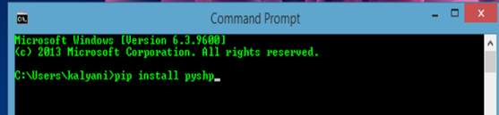
Fig 7.1
- Then we perform the installation of Python libraries namely pyshp, pyqtree and Matplotlib – which will be used in order to load the shape files and visualize them as shown in Fig. 7.2
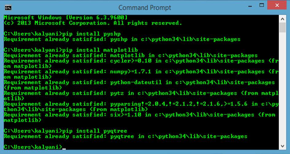
Fig 7.2
- The Fig 7.3 displays the geo-spatial data source where the data is present in shapefile format and also in other format like .csv for the purpose of further analysis.
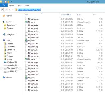
Fig 7.3
- As shown in Fig. 7.4, then we start coding in python platform to store the data.
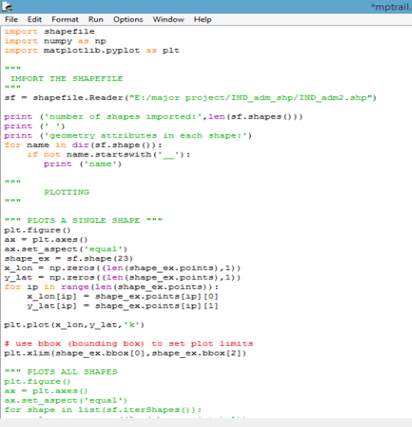
Fig 7.4
- We then require Matplotlib functions as shown in Fig. 7.5 in order to plot the data corresponding to the bounding box attributes thus to visualize the data.
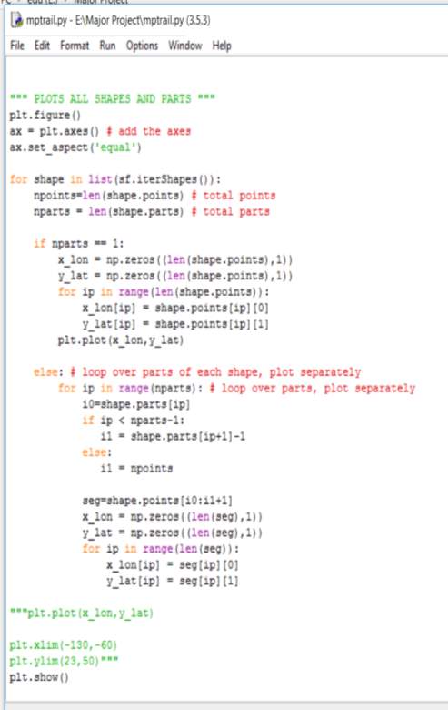
Fig 7.5
- After writing the Python code, we need to run the code to observe the expected output. The command used for running the code is python filename.py.
Fig 7.6
- After observing the output by running Python code, we need to establish the connection between R and Python and the first step to do so is to install the developer tools (devtools) as shown in Fig. 7.7.
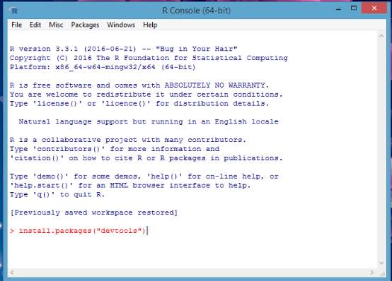
Fig 7.7
- To install the packages in R we need to select the CRAN mirror to initiate the installation, as shown below in Fig 7.8.
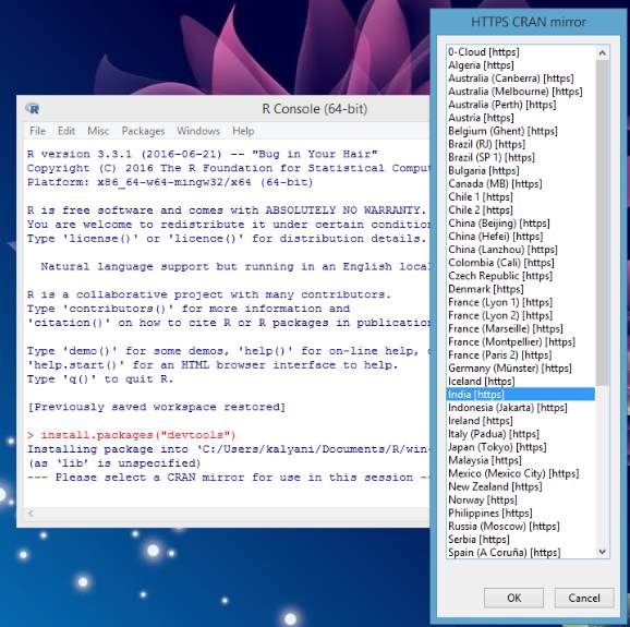
Fig 7.8
- For the effective working of the R packages we need to install Rtools along with devtools. Fig. 7.9 displays the Rtools installation setup.
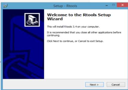
Fig 7.9
- The step shown in Fig. 7.10 depicts the installation of various libraries and packages in association with the devtools in order to support the efficient working of the other packages.
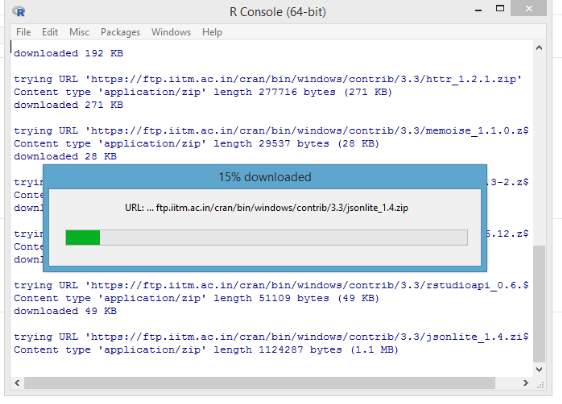
Fig 7.10
- Fig. 7.11 shows the completion of the setup of Rtools.
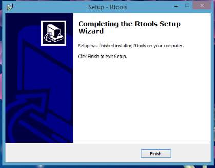
Fig 7.11
- The step shown in Fig. 7.12 depicts the usage of devtools which is initiated by the command library (package name).
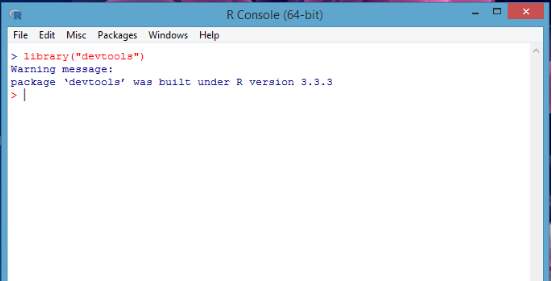
Fig 7.12
- One of the problems encountered when transferring the data from Python to R is the output from Python is in the JSON format, which is unaccepted by R. Hence as shown in Fig. 7.13 we install RJSONIO package to convert the input data into R.
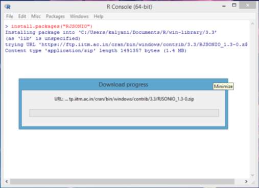
Fig 7.13
- As shown in the below Fig 7.14, we need to use the rPython-win package to form the interface between R and Python after the installation RJSONIO.
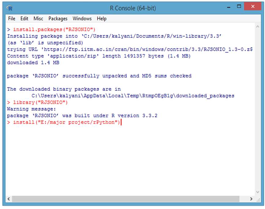
Fig 7.14
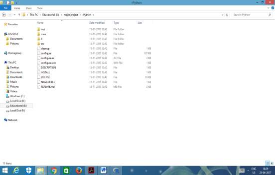 This step as shown in Fig. 7.15 depicts the contents of rPython-win package.
Fig 7.15
- We need to modify the configure.win file which contains the path to Python, so that it directs to the exact location of the Pytrhon files as shown in Fig. 7.16.
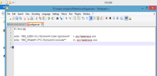
Fig 7.16
- In the below Fig 7.17, after loading the rPython library, we are executing the Python code from R console using the command “python.load (“destination address”)”.
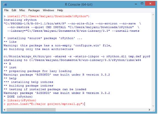
Fig 7.17
- Below shows the visualization of the analysis of shapefiles retrieved from the R platform which is the expected output of the project.
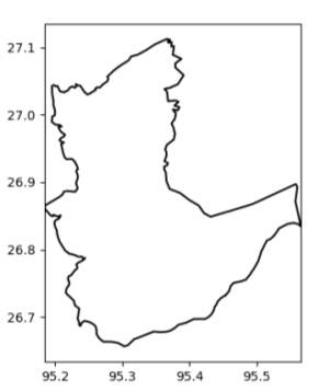
Fig 7.19
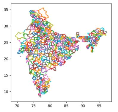
Fig 7.2
CHAPTER 8
CONCLUSION AND FURTHER SCOPE
CONCLUSION AND FURTHER SCOPE
8.1 CONCLUSION
Geo-spatial Data Analysis can be used anywhere in the world to derive the conclusion regarding spatial data stored in trees. Hence the project concludes that by using the model for analysing the geo-spatial data, users will be able to attain productive solutions to unknown factors based on the known constraints using Data Mining Algorithms and thus visualising the outcome on the maps.
The feature of accessing the data from the maps might seem little odd in the beginning but it has numerous advantages which can make the life of beings easy and qualitative. It would become easy to locate the places where the administrative buildings are in each state as well as get their co-ordinates and plot them. Furthermore, this plotting of the shapefiles produces illustrative maps which can make the process of visualization easy and reliable. The interface that has been developed between R and Python will help the developers and analysts to utilize the packages in both the platforms and render the data in effective way, thus the package building is not restricted to one platform but is multi-platform based.
Thus, in this project We store the Geo-spatial data from the maps into trees and then import the data in the format of shapefiles. In Python, we store the shapefiles using bounding box as the boundary, then the data is analyzed and visualize the results onto map. Then the interface between R and Python is established with the help of rPython- win package. The features of the system are probabilistic, reliable and useful due to the application in Real Time. The project’s outcome is to depict the plots of the spatial data with the physical boundaries as well as the individual state information when the shape number of the shape is provided. Here the advancement of the geographic information system is provided where the geography of the entire country is depicted in various colors, making the user to precisely understand the topographic nature of the place and if further extended it helps the people to collaborate with their respective fields to reach clear results.
8.2 FUTURE SCOPE
Geospatial data, this is where the future of many unforeseen technologies rely on. This is not an independent specialization where we can use just for maps and roads, but when this is collaborated with different domains the results generated will put the world to surprise and is the next sighted solution for many problems. There is a possible extension to the project by clipping the regions in the CSV file onto the plotted map, thus it depicts the plot in a clear and concise manner to the users.
BIBLIOGRAPHY
- https://github.com/ArmchairArmada/python-quadtree/blob/master/quadtree.py
- https://geohackweek.github.io/vector/04-geopandas-intro/
- http://statweb.stanford.edu/~tibs/ElemStatLearn/
- http://www.code-spot.co.za/downloads/python_image_code/doc/html/classquadtree_1_1_quadtree.html
- http://dx.doi.org/10.1109/mwscas.2011.6026611
- https://gist.github.com/acrosby/4601257
- http://pythonhosted.org/Pyqtree/#header-classes
- https://chrishavlin.wordpress.com/2016/11/16/shapefiles-tutorial/
- https://pypi.python.org/pypi/pyshp
- http://www.datadependence.com/2016/06/creating-map-visualisations-in-python/
- https://www.r-bloggers.com/integrating-python-and-r-into-a-data-analysis-pipeline-part-1/
- https://sites.google.com/site/aslugsguidetopython/data-analysis/pandas/calling-r-from-python
- https://github.com/cjgb/rPython-win
- http://www.di.fc.ul.pt/~jpn/r/langs/python.html
- https://cran.r-project.org/web/views/Spatial.html
- http://toblerity.org/rtree/
- https://libspatialindex.github.io/index.html
- http://toblerity.org/rtree/install.html#installation
- S. Palaniappan, Dr. T. V. Rajinikanth, Dr. A. Goverdhan Spatial Data Analysis using various Tree classifiers ensembled with AdaBoost Approach, Emerging trends in Electrical, communications and Information Technology.
- S. Palaniappan1, T. V. Rajinikanth and A. Govardhan Enhancement of Effective Spatial Data Analysis using R, Indian Journal of Science and Technology, Vol 9(21).
- Rajanikanth J, Rajinikanth TV, Prasad TVKP, Radha Krishna B. Analysis on Spatial Data Clustering Methods – A Case Study. 2012 Oct- Dec; 3(4):51–4.
- L. Arge, M. de Berg, H. J. Haverkort, and K. Yi. The priority R-tree: A practically efficient and worst-case optimal R-tree. In Proceedings of ACM Management of Data (SIGMOD), pages 347–358, 2004.
- N. Beckmann, H. Kriegel, R. Schneider, and B. Seeger. The R*-tree: An efficient and robust access method for points and rectangles. In Proceedings of ACM Management of Data (SIGMOD), pages 322–331, 1990.
- Y. J. Garcia, M. A. Lopez, and S. T. Leutenegger. On optimal node splitting for r-trees. In
Proceedings of Very Large Data Bases (VLDB), pages 334–344, 1998.
- A. Guttman. R-trees: a dynamic index structure for spatial searching. In Proceedings of ACM Management of Data (SIGMOD), pages 47–57, 1984.
- I. Kamel and C. Faloutsos. Hilbert R-tree: An improved R-tree using fractals. In Proceedings of Very Large Data Bases (VLDB), pages 500–509, 1994.
- T. K. Sellis, N. Roussopoulos, and C. Faloutsos. The R+-tree: A dynamic index for multi-dimensional objects. In Proceedings of Very Large Data Bases (VLDB), pages 507–518, 1987.
- M Astrahan, et aI , System R* Relational Approach to Database Management, AC.@ Runsactzons MZ Database &stems 1, 2 (June 1976), 97-137.
- R Bayer and E McCrelght, Organization and Maintenance of Large Ordered Indices, Proc 1970 ACM-SIGFTDET Workshop on Data lkscrzphon and Access, Houston, Texas, Nov. 1970, 107-141.
- J L Bentley, Multidimensional Binary Search Trees Used for Associative Searching, Communications of the ACM 18,9 (September 1975) 509517.
Cite This Work
To export a reference to this article please select a referencing stye below:
Related Services
View all


Related Content
All TagsContent relating to: "Technology"
Technology can be described as the use of scientific and advanced knowledge to meet the requirements of humans. Technology is continuously developing, and is used in almost all aspects of life.
Related Articles

DMCA / Removal Request
If you are the original writer of this dissertation and no longer wish to have your work published on the UKDiss.com website then please: