Relationship Between Particle Size Distribution and the Sealing Efficiency of Lost Circulation Materials
Info: 12834 words (51 pages) Dissertation
Published: 17th Dec 2019
Tagged: EngineeringSciences
Abstract
Lost circulation of drilling fluid is considered as the worst nightmare to be faced while drilling for hydrocarbons. However; the invention of lost circulation materials (LCMs) helped overcoming this problem. LCMs are often used as a corrective approach to mitigate the fluid losses into the formation. Previous studies concluded that particle size distribution (PSD) was found to be one of the essential parameters that improves the sealing efficiency of LCM treatments.
Thus, in this study, we will try to understand the relationship between PSD and the sealing efficiency of LCMs. Our experiments were conducted using a slotted disc with a known width to simulate fractures. Different formulations of LCM treatments will be evaluated experimentally under low pressure using the standard API filter press to investigate the effectiveness of the formulated treatments in sealing fractures. PSD analysis will be conducted using dry sieve analysis techniques to understand the relationship between PSD and the sealing efficiency.
1.1.1 Drilling fluids can be classified into three main types:
1.1.2 Lost circulation problems during drilling operations
1.2 Classifications of Fractured Formations
1.3 Loss Circulation Treatments
2.1 LCM Performance Evaluation Tests.
3.2 Particle Size Distribution Analysis
3.2.2 Test Procedure for Sieve Analysis
3.3 LCM Performance Evaluation
3.3.2 Conventional LCM’s Used.
3.3.2 Conventional LCM’s Used.
3.4 Low-pressure low-temperature (LPLT) LCM Testing
3.4.1 Fracture Width Variation
4.1 [15ppb] LCM Fluid Losses Results:
4.2 [50ppb] lcm Fluid losses results:
4.3 [15ppb] Control Samples fluid loss Results
4.3 The Effect of Viscosity on Sealing Efficiency:
4.5 Particle size Distribution:
4.5.1 Test sample LCM #1 sieve analysis:
4.5.2 Test sample LCM #2 sieve analysis:
4.5.3 Test sample LCM #3 sieve analysis:
4.5.4 Test sample LCM #4 sieve analysis:
4.5.5 Test sample LCM #5 sieve analysis:
4.5.6 Test sample LCM #6 sieve analysis:
4.5.7 Nut Shells sieve analysis:
5.1 Effect of concentration in fluid loss
6. Conclusion and Recommendations
List of Figures
Figure 1 illustration on Types of fractures (GEORGE C. HOWARD and P. P. SCOTT, April 12,1951)
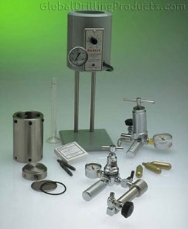
Figure 2 Particle Plugging Apparatus (OFITE, n.d.)
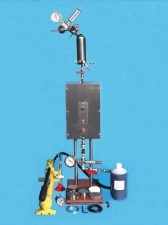
Figure 3 HPHT filter press (FANN Testing Equipment, n.d.)
Figure 4 Low Pressure LCM Test (Alsaba, 2015)
Figure 5 Endecotts EFL 2000 Sieve Shaker
Figure 9 5 Bench-Mount LPLT Filter Press (OFITE, n.d.)
Figure 10 The manufactured spacer
List of Tables
Table 1 LCM’s Categorization (Darley and Gray 1988)
Table 2 Sieve Analysis Test Sample
Table 3 Drilling fluid properties
Table 4 LCM formulations at 15 ppb concentration
Table 5 LCM formulations at 50 ppb concentration
Introduction
With the growing of energy demand and the growing numbers of depleted reservoirs in the world, the oil and gas industry is now shifting its focus into unconventional and challenging wells, this type of operations are usually very expensive in term drilling operations, which means any drilling non-productive time (NPT) can cause a significant economic impact, and one of the biggest contributor to drilling NPT is lost circulation events, which can be defined as the loss circulation of drilling fluids into the formation.
1.1 Drilling Fluid
Drilling fluids can be defined as the fluids that are used during the drilling of subterranean wells. They provide primary well control of subsurface pressures by a combination of density and any additional pressure acting on the fluid column (annular or surface imposed). They are most often circulated down the drill string, out the bit and back up the annulus to the surface so that drill cuttings are removed from the wellbore. (IADC Drilling Manual, 2014)
Drilling fluid functions as a mean to transport drilling cutting to the surface, also can be used to Clean, cool and lubricate the drill bit, provide hydrostatic pressure to control the well while drilling, prevent excessive mud loss while drilling, transmit hydraulic horsepower to the bit, Prevent formation damage.
1.1.1 Drilling fluids can be classified into three main types:
Water-base mud (WBM): WBM is a drilling fluid where water is the continuous phase. It is safe and economical and that’s why it is the most common drilling fluid where it has been used to drill approximately 80% of all oil wells. (Spears & associates, 2004)
Types of WBM:
- Non-dispersed inhibited
- Dispersed non-inhibited
- Dispersed inhibited
Oil-base mud (OBM): OBM is drilling fluid where oil is the continuous phase. It is effective when increasing the penetration rate is intended. In addition; it could be used in special cases such as drilling though high pressure or high temperature formations. Moreover; using OBM is convenient when drilling though shale by which it prevents shale swelling. However, it has a potential to cause health problems to those works in site, contaminate soil, and ground water aquifers. (Advances in Petroleum Exploration and Development, 2011)
Types of OBM:
- Invert emulsion oil muds
- Pseudo oil based mud
Pneumatic-drilling fluids: Compressed air or gas can be used in place of drilling fluid to circulate cuttings out of the wellbore. Pneumatic fluids fall into one of four categories:
Types of Pneumatic fluid: –
- Air
- Mist
- Foam
- Aerated drilling fluid
specialized equipment’s are used in pneumatic drilling to help and ensure the return of cuttings and formation fluids to the surface, in addition to compressor, tanks, valve and lines with the association of gas that is used for drilling.
One of the disadvantages of using pneumatic drilling fluid is when drilling through high pressure and high temperature formation which demand high density fluid in order to avoid well control issues. However, using pneumatic fluids offers several advantages: (S.A.), 1999)
- minimal formation damage.
- Easier to evaluate the presence of hydrocarbon through the cuttings.
- Prevention of lost circulation.
- In hard formations allow higher penetration rates.
There are many drilling fluid additives which are used to change the mud weight or chemical properties such as:
- Weighting materials which are compounds that are dissolved in the drilling fluid to increase its density. They are used to control the formation pressures; Example of weighting materials; Bentonite, Barite, Hematite and Calcite
- Viscosifiers can be defined as materials that are used to increase the viscosity of drilling fluid; examples (Clays and Polymers)
Adding clays to water will enhance the drilling mud viscosity and yield point properties which will improve its ability to left the cuttings.
Polymers are used as a borehole stabilizing agent to prevent swelling. Moreover; when we add it to bentonite based drilling mud, it will increase gel strength, resulting suspension of coarse drill cuttings.
Most common hazards in drilling that can be overcome by proper control of the drilling fluid properties:
Salt section hole enlargement
Such a hazard is caused by the erosion of salt section of formation as a result of being in contact with the drilling fluid causing hole enlargement. To overcome such a problem a salt saturated mud system is prepared prior drilling into a salt formation.
Heaving shale problems
Shale formations containing bentonite and other types of clays tend to continually absorb water resulting a swelling and slough into the borehole which will eventually cause pipe sticking and solid build up in the mud.
This problem can be treated in different ways such as changing the mud system to high calcium content which has the tendency to reduce the tendency of mud to hydrate water sensitive clay. Other solutions to this problem are to either use oil base mud instead of water base mud to avoid any water absorption by formation or increase the mud density for greater wall support.
1.1.2 Lost circulation problems during drilling operations
Lost circulation means the loss of drilling fluid into naturally fractured or drilling induced fractured formations, in other words; the situation where less drilling fluid is returned to surface than is pumped into subsurface causing a major reduction in hydrostatic pressure which will cause the fluids in the formation to flow into the well bore resulting in kicks (www.wildwell.com/literature-on-demand/literature/causes-of-kicks.pdf) .
Moreover; a sever loss of circulation could cause what it’s called dry drilling, which could result undesired damaging of formation and destruction of drill bit. (infohost.nmt.edu/~petro/faculty/Kelly/Drilling%20Problems.pdf)
Thus, when loss of circulation does occur new requirements of time and mud or cement will be added enormously to the overall cost of a well. Such a problem could be prevented or mitigated using bridging or plugging materials (loss of circulation materials) which are capable of sealing these fractures existing in the formation.
Economic impact of loss circulation can be evaluated in term of nonproductive time and the high cost of lost drilling fluid, where some estimates stated that the annual cost of loss of circulation including the cost of materials and rig time is around one billion dollars worldwide. And also, it’s worth to mention that according to some estimates, the cost of drilling fluid laying between 25% -40% of the total drilling cost, which is really considerable amount of money will be spent if loss of circulation occurred. (Lavrov, 2016)
The losses can lead to sever consequences depending on the amount of fluid losses. And the losses can be classified based on the rate of fluid lost in
bblhr:
- Seepage (1-10
bblhr)
- Partial (10 to 500
bblhr)
- Sever (>500
bblhr)
1.2 Classifications of Fractured Formations
One of the factors that control the fluid loss severity is the type of formations in which the fluid enters, and these types of fractured formations can be classified as:
- Natural Fracture (Fig.1 a)
- Induced Fracture (Fig.1 a)
- Cavernous Fracture (Fig.1 b)
- Unconsolidated or Highly Permeable Formations (Fig.1 c)
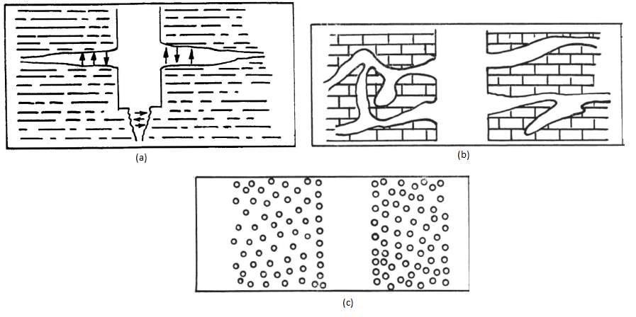
Figure 1 illustration on Types of fractures (GEORGE C. HOWARD and P. P. SCOTT, April 12,1951)
For fluid loss to occur in natural fractures requires only sufficient pressure to exceed that of the fluid within the formations. While induced fractures, requires that the fluid pressure should be sufficient in magnitude to fracture the formation.
Another form of fractures, which is cavernous fractures, occurs when mud pressure exceeds the formations pressures (Fig. 1c).
For drilling fluid to be lost in unconsolidated formations, requires the intergranular passages to be large enough to allow the mud to enter the formations. (GEORGE C. HOWARD and P. P. SCOTT, April 12,1951)
1.3 Loss Circulation Treatments
By addressing the loss severity and the type of formation fracture, proper treatment can be applied to mitigate or even prevent the losses. And as for the LCM’s treatments, there are two types of treatments that are primarily depend on the occurrence time of loses.
Corrective Treatments. It’s basically like any method that is applied after the occurrence of losses. With the corrective treatment, the loss circulation materials are added continually to the drilling mud or as concentrated pills to reduce the losses. There are two type of LCM’s; conventional and unconventional, the conventional LCM’s can be defined as the solid particles that is suspended within the drilling fluid to prevent losses, and these particles can be classified based on their physical properties and their appearance in four categories [granular, fibrous, flaky and a mix blend of the three] (Howard and Scott, 1951; White, 1956; Canson, 1985). As mentioned before, there are three type of fluid losses; seepage, partial and sever losses and the conventional LCM treatments are usually used to control and mitigate seepage or partial losses, however, for severe loses unconventional LCM’s (ex. LCM pills) are used to fill and bridge fractures.
Preventive Treatments its can be basically defined as the treatment applied prior the occurrence of fluid losses or entering a lost circulation zone to prevent any losses, the main objective for this treatment is to strengthen the well (Whitfill, 2008). Wellbore strengthening is basically a set of techniques that are used to plug and seal induced fracture efficiently while drilling (Salehi and Nygaard, 2012).
2. Literature Review
The main objective of this section is to review different available tests that evaluate loss circulation materials (LCM) performance, discuss bridging theories and finally there will be a brief critical review on the literature.
2.1 LCM Performance Evaluation Tests.
There are different parameters that are measured to indicate the performance of LCM’s. Evaluating the performance of LCM’s prior field application is an important step to optimize the effectiveness of the treatment.
To evaluate the performance of LCM’s as corrective approach there are two commonly used testing apparatuses as a standardized test which are; High-Pressure High-Temperature (HPHT) filter press (Figure 3) and Particle Plugging Apparatus (PPA) (Figure 2), these tests are conducted using earthier slotted discs or tapered discs to simulate fractures that are natural or induced (Alsaba, 2015). HPHT filter press and particle plugging test are used to serve the same purpose which is to determine the ability of the fluid to effectively bridge the fractured discs under constant pressure and temperature, but with one main difference between them is that the PPA is modified to operate upside down (pressure applied from bottom) as shown in figure 2 to eliminates the effects of gravity.
Low Pressure LCM Test is Another type of LCM evaluating test which was manufactured based on API filter Press (Alsaba, 2015) and it contained tapered discs with a-snug fit spacer as shown in the (Figure 4) below, the spacer served as a holder for the tapered discs also, to prevent the cell outlet from being plugged, the test was run at 100 psi with basic WBM and the LCM’s, by applying the pressure the fluid will start flowing through the tapered discs and fluid will start coming out, this test highlighted the fluid loss volume, which can be affected by other parameters such as concentration and particle size distribution which helps in sealing fractures.
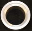
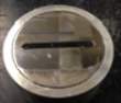
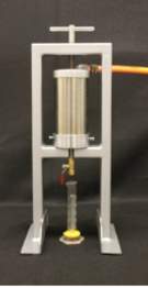
Figure 4 Low Pressure LCM Test (Alsaba, 2015)
2.2 Bridging Theories.
Over the past 40 years there has been immense developments on how to improve the bridging capabilities of drilling fluid, bridging is defined as the restriction of fluid losses into formation by building up fluid solids within the fracture or pore spaces which leads to the reduction of formation damage that can be caused by the fluid losses into the formation.
In 1977, Abrams proposed two rules to optimize the selection of PSD and concentration to minimize the fluid losses into the formation. The first rule was on the average particle size, where the D50 should be
13of the formation pore size. The second rule proposed that upon choosing the bridging material the concentration should be equal or larger than 5% of the total solids in the drilling fluid.
Another criterion done by Smith in 1996 for the selection of PSD based on his field observation that led to the reduction of formation damage and the increase of production rates. The criteria suggested that the D90 of PSD of the used bridging material should equal to the pores size to minimize the losses of drilling fluids into the formation.
In 2008 Whitfill proposed a new method based on fracture widths and PSD, the method is based of fracture width rather than pores. This method proposed that the D50 value should be equal to the fracture width to ensure that the fracture is effectively sealed.
And most recently in 2016, an updated criterion was proposed by Alsaba et al. 2016 based on laboratory investigations to develop and enhance the bridging capabilities of drilling fluids. The criteria proposed that the D50 values should be equal or greater than
310of the fracture width and the D90 values should be equal or greater than
65 of the fracture width to effectively seal fractures.
2.3 Critical Review.
The literature review of the LCM performance evaluation has shown the different parameters that can indicate the fluid loss volume and the sealing efficiency through different testing apparatuses. Both HPHT test and PPA test where used to evaluate the ability of the fluid to seal the fracture under constant temperature and pressure, while the LP test was used to the determine the fluid loss volume that is affected by the concentration and PSD.
The development of bridging theories has revealed the improvement of bridging capabilities of the drilling fluid. The development of bridging theories with their selected criterions were aimed towards optimizing the selection PSD as well as concentration. Whitfill have proposed a method based on PSD and fracture widths. However, this criterion has been updated as of recent by Alsaba et al. which was based on Laboratory investigations.
2.4 Report Objectives
The main objective of this research is to:
- Try to prove that particle size distribution is one of the major parameters that improve sealing efficiency.
- Understand the relationship between particle size distribution and the sealing efficiency.
- Investigate the impact of loss circulation materials properties and concentration on sealing efficiency.
- Investigate the effectiveness of the formulated treatments in sealing fractures.
By establishing a firm relationship between PSD and sealing efficiency based on specific fracture width not only will aid in selecting effective LCM treatment but also, to mitigate or even prevent fluid losses.
3. Methodology
This chapter will cover the methodologies used to accomplish the objectives set in the previous chapter. Furthermore, this chapter will include any experiments, data analysis, procedures and materials used in this project.
LCM’s appear in large numbers and are used in various applications. Therefore, it is very important to test the LCM’s and classify them. Dry sieve analysis techniques were used to analyze the particle size distribution (PSD) of LCM treatment to find how PSD can affect the sealing pressure and fracture sealing for the desired fracture width. Those analyses can help determine the role of effective blends and the role of PSD in having an effective fracture sealing and therefore, determine the best selection that can provide the best sealing efficiency.
Finally, this section covers the apparatus that is used to evaluate the performance of LCM’s in this project, which is the low-pressure low-temperature filter press (LPLT).
LCMs are usually classified by their shapes into flaky, granular, and fibrous materials (Darley and Gray 1988). Sometimes, materials of different shape are mixed together to create a mixed-shape blend (White 1956). Table 1 below shows the categorization of the different shapes of LCM’s.
Table 1 LCM’s Categorization (Darley and Gray 1988)
| Flaky | Granular | Fibrous |
| Cellophane | Calcium carbonate | Asbestos |
| Cotton seed hulls | Coal | Bagasse |
| Mica | Diatomaceous earth | Flax shives |
| Vermiculite | Nut shells | Hog hair |
| Olive pits | Leather |
Traditionally, there are three particle size determination methods: Sieve analysis, and the sedimentation method (Darley and Gray 1988). The method used to estimate the PSD for this project is: dry sieve analysis. The sieve analysis is performed by shaking of materials through a set of sieves with smaller openings. Sieve analysis usually involves human error and is time consuming. However, sieve analysis was the only method that was available to use for this project. The sieve shaker used for the LCM samples is the Endecotts EFL 2000 Sieve Shaker (Fig. 5). Results obtained from the sieve analysis are represented in which the percentage of the total weight of the sample that passed through the different sieves. The parameters for the blends used for the fracture widths are the D50, D70 and D90 based on the PSD selection criterion of proposed by Alsaba et al. 2016. Figure 1 below shows the sieve shaker that was used to perform the test.
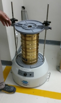
Figure 5 Endecotts EFL 2000 Sieve Shaker
Table 2 below represents a sample of the sieve analysis test. The sieve sizes were chosen based on the particle sizes that we are dealing with. The largest particle doesn’t’ exceed 4.75mm, therefore Sieve # 4 (4.75mm) is largest sieve chosen.
Table 2 Sieve Analysis Test Sample
| Sieve # | Sieve Size (mm) | Empty Weight (g) | Weight after Shake (g) | Weight of retained Particles (g) | % Retained | Cumm. Retained % | % Finer |
| 4 | 4.75 | 750.9 | |||||
| 8 | 2.36 | 444.3 | |||||
| 16 | 1.18 | 634.3 | |||||
| 30 | 0.60 | 601.6 | |||||
| 40 | 0.43 | 334.7 | |||||
| 50 | 0.30 | 535.9 | |||||
| 100 | 0.15 | 508.2 | |||||
| 200 | 0.08 | 489.5 | |||||
| Pan | 0.01 | 473.4 | |||||
| Sum (g) |
3.2.2 Test Procedure for Sieve Analysis
The procedure is as follows:
- Sieves selected were checked if they are cleaned prior the test.
- Each sieve selected was weighted, including the pan.
- The sieves are then stacked up and placed on top of each other, starting from the pan at the bottom, to the largest sieve size at the top.
- The LCM formulation samples is poured into the sieve stack and the sieve is manually shook to make sure the sample travels through the sieves.
- The sieve is then placed on the sieve shaker machine for 30 minutes (API STD).
- Once the time is up, the machine is then stopped and the sieve stacks are removed from the shaker.
- each sieve is then weighted and written down on a results page.
- % of the retained of sieves is calculated using this formula:
Weight of particles retained2
- Cumulative % retained calculated using this formula:
∑% Retained
- % finer is calculated from this formula:
100%- ∑% Retained
3.3 LCM Performance Evaluation
This will include the drilling fluid that is used in this project and its properties as well as the formulations of the LCM’s used.
The fluid used in this project is a water-based mud that consists of 325ml water and 7% of bentonite (25ml) that aims to diminish any effects (negative or positive) of other drilling fluid additives. Rheology and PH tests were performed on this fluid to get the density, gel, and viscosity and yield point. The tests were applied on a fresh mud sample as well as a viscous mud sample (which was mixed and stored for one week to get full bentonite hydration) to create a comparison. Table 3 below shows the measured properties of the drilling fluid.
Table 3 Drilling fluid properties
| Fresh mud sample | Viscous mud sample | |
| Density (PPG) | 8.6 | 8.6 |
| Readings @300 RPM | 27 | 42 |
| Readings @600 RPM | 30 | 44 |
| Gel strength after 10 sec (lb/100 ft2) | 21 | 34 |
| Gel strength after 10 min (lb/100 ft2) | 24 | 36 |
| Plastic Viscosity (cp) | 3 | 2 |
| Apparent Viscosity (cp) | 15 | 22 |
| Yield Point (YP) (lb/100 ft2) | 24 | 40 |
| PH | 9.57 | 9.5 |
Plastic Viscosity (PV) = Reading at 600 rpm – Reading at 300 rpm in cp
Apparent Viscosity (AV) = Reading at 300 rpm
Yield Point (YP) = Reading at 300 rpm – Plastic Viscosity (PV) in lb/100 ft2.
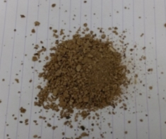
3.3.2 Conventional LCM’s Used.
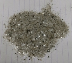
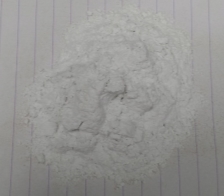
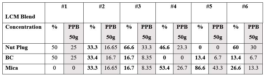
The conventional LCM’s used in this project are: Baracarb 50, Nutshells, and Mica. Those are the only LCM’s available to us for the project. The formulations were created (randomly) using the above LCM’s at a concentration 15ppb, which represents background treatments, and at concentration of 50 ppb, which represents concentrated LCM pills. Table 4 and 5 below shows the LCM formulations at both the 15 ppb and 50 ppb concentrations.
3.3.2 Conventional LCM’s Used.
The conventional LCM’s used in this project are: Baracarb 50, Nutshells, and Mica. (Figure #, #, # shows the materials used in this project.) Those are the only LCM’s available to us for the project.
The formulations were created (randomly) using the above LCM’s at a concentration 15ppb, which represents background treatments, and at concentration of 50 ppb, which represents concentrated LCM pills. Table 4 and 5 below shows the LCM formulations at both the 15 ppb and 50 ppb concentrations.
Table 4 LCM formulations at 15 ppb concentration
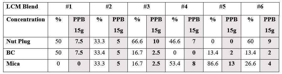
Table 5 LCM formulations at 50 ppb concentration
3.4 Low-pressure low-temperature (LPLT) LCM Testing
The low-pressure apparatus used in our project is the bench-mount filter press, which is based on the API filter press design. Figure 3 below shows the filter press that was used during this project.
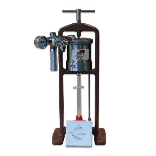
Figure 9 5 Bench-Mount LPLT Filter Press (OFITE, n.d.)
We’ve managed to manufacture our own spacer (shown in the figure below) which served as a holder for the discs to prevent plugging the cell outlet. The spacer has an outside diameter of 79mm and an inside diameter of 60mm, and a thickness of 1 inch (25.4mm).
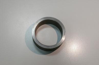
Figure 10 The manufactured spacer
3.4.1 Fracture Width Variation
Three slotted discs were created in the carpenter with different fracture width. The fracture widths are 1000 microns, 1500 microns and 2000 microns. We have faced difficulties with manufacturing the 500 microns’ fracture width and therefore, we decided to use the above sizes only. Figure 2 below shows the three discs that were used. Table 5 below shows the disc’s specifications.
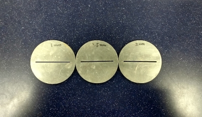
Figure 7 The three slotted discs used for filter press test
| Disc No. | Diameter (mm) | Thickness (mm) | Fracture Aperture (microns) |
| Disc 1 | 8 | 0.6 | 1000 |
| Disc 2 | 8 | 0.6 | 1500 |
| Disc 3 | 8 | 0.6 | 2000 |
The procedure is as follows:
- Mud sample is with 325ml water and 25g bentonite is prepared prior the test.
- LCM formulation is poured and mixed with the prepared mud sample.
- Gasket is inserted into the base and attach into the cylinder. The connection needs to be checked in case of a loose fit.
- The volume of the fluid sample needs to be measured before pouring it in the cell.
- The fluid sample is poured into the cell.
- The pressure cap is then sealed on top of the cell and tighten securely.
- A graduated cylinder is then Placed under the cell filtrate tube.
- The regulator is then turned on and the pressure gradually increased.
- A timer is set on to measure the sealing time.
- The pressure regulator is then Turned off once the test is done and the pressure released from the cell.
- The top assembly is remove and the cell is emptied into a container.
- the fluid loss volume is measured and written down as results.
4. Results
4.1 [15ppb] LCM Fluid Losses Results:
| LCM Blend | #1 | #2 | #3 | #4 | #5 | #6 | |||||||
| Concentration | % | PPB 15g | % | PPB 15g | % | PPB 15g | % | PPB 15g | % | PPB 15g | % | PPB 15g | |
|
Nut Plug |
50 |
7.5 |
33.3 |
5 |
66.6 |
10 |
46.6 |
7 |
0 |
0 |
60 |
9 |
|
|
BC |
50 |
7.5 |
33.4 |
5 |
16.7 |
2.5 |
0 |
0 |
13.4 |
2 |
13.4 |
2 |
|
|
Mica |
0 |
0 |
33.3 |
5 |
16.7 |
2.5 |
53.4 |
8 |
86.6 |
13 |
26.6 |
4 |
|
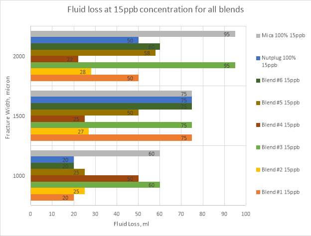
| Fluid loss at 1000 micron |
20 ml |
25 ml |
60 ml |
50 ml |
25 ml |
20 ml
|
|||||||
| Fluid loss at 1500 micron |
75 ml |
27 ml |
75 ml |
25 ml |
50 ml |
75 ml
|
|||||||
| Fluid loss at 2000 micron |
50 ml |
28 ml |
95 ml |
22 ml |
58 ml |
60 ml
|
|||||||
4.2 [50ppb] lcm Fluid losses results:
| LCM Blend | #1 | #2 | #3 | #4 | #5 | #6 | |||||||
| Concentration | % | PPB 50g | % | PPB 50g | % | PPB 50g | % | PPB 50g | % | PPB 50g | % | PPB 50g | |
|
Nut Plug |
50 | 25 |
33.3 |
16.65 |
66.6 |
33.3 |
46.6 |
23.3 | 0 | 0 |
60 |
30 | |
|
BC |
50 | 25 |
33.4 |
16.7 |
16.7 |
8.35 | 0 | 0 |
13.4 |
6.7 |
13.4 |
6.7 | |
|
Mica |
0 | 0 |
33.3 |
16.65 |
16.7 |
8.35 |
53.4 |
26.7 |
86.6 |
43.3 |
26.6 |
13.3 | |
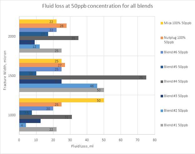
| Fluid loss at 1000 micron |
22 ml |
4 ml |
12.5 ml |
31 ml |
7.5 ml
|
20 ml |
|||||||
| Fluid loss at 1500 micron |
50 ml
|
46 ml |
25 ml |
75 ml |
10 ml
|
25 ml |
|||||||
| Fluid loss at 2000 micron |
25 ml |
12 ml |
9 ml |
35 ml
|
17 ml |
22 ml |
|||||||
| LCM Blend | NP | NP | Mica | Mica | ||||
| PH | 6.85 | 6.8 | 9.35 | 9.5 | ||||
| Concentration | % | PPB 15g | % | PPB 50g | % | PPB 15g | % | PPB 50g |
| Nut Plug | 100 | 15 | 100 | 50 | 0 | 0 | 0 | 0 |
| BC | 0 | 0 | 0 | 0 | 0 | 0 | 0 | 0 |
| Mica | 0 | 0 | 0 | 0 | 100 | 15 | 100 | 50 |
| Fluid loss at 1000 micron | 20 ml | 25 ml | 60 ml | 50 ml | ||||
| Fluid loss at 1500 micron | 75 ml | 27 ml | 75 ml | 25 ml | ||||
| Fluid loss at 2000 micron | 50 ml | 28 ml | 95 ml | 22 ml | ||||
4.3 [15ppb] Control Samples fluid loss Results
4.3 The Effect of Viscosity on Sealing Efficiency:
| LCM Blend | #1 | #2 | #3
Not sure if its viscous or not |
|||
| Concentration | % | PPB 15g | % | PPB 15g | % | PPB 15g |
|
Nut Plug |
50 |
7.5 |
33.3 |
5 |
66.6 |
10 |
|
BC |
50 |
7.5 |
33.4 |
5 |
16.7 |
2.5 |
|
Mica |
0 |
0 |
33.3 |
5 |
16.7 |
2.5 |
| Fluid loss at 1000 micron |
2 ml |
4 ml |
25 ml |
|||
| Fluid loss at 1500 micron |
8 ml |
25 ml |
75 ml |
|||
| Fluid loss at 2000 micron |
28 ml |
26 ml |
95 ml |
|||
4.5 Particle size Distribution:
4.5.1 Test sample LCM #1 sieve analysis:
| Sieve # | Sieve Size (mm) | Empty Weight (g) | Weight after Shake (g) | Weight of retained Particles (g) | % Retained | Cumm. Retained % | % Finer |
| 4 | 4.75 | 750.9 | 751 | 0.1 | 0.2 | 0.2 | 99.8 |
| 8 | 2.36 | 444.3 | 449.8 | 5.5 | 11 | 11.2 | 88.8 |
| 16 | 1.18 | 634.3 | 649.1 | 14.8 | 29.6 | 40.8 | 59.2 |
| 30 | 0.60 | 601.6 | 604.7 | 3.1 | 6.2 | 47 | 53 |
| 40 | 0.43 | 334.7 | 335.3 | 0.6 | 1.2 | 48.2 | 51.8 |
| 50 | 0.30 | 535.9 | 536.4 | 0.5 | 1 | 49.2 | 50.8 |
| 100 | 0.15 | 508.2 | 510 | 1.8 | 3.6 | 52.8 | 47.2 |
| 200 | 0.08 | 489.5 | 495.6 | 6.1 | 12.2 | 65 | 35 |
| Pan | 0.01 | 473.4 | 490.7 | 17.3 | 34.6 | 99.6 | 0.4 |
| Sum (g) | 4822.6 | 49.8 |

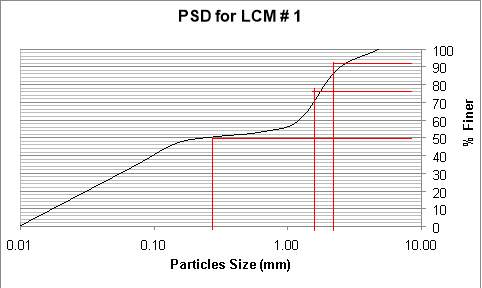
| mm | microns | |
| D(50) | 0.28 | 280 |
| D(75) | 1.8 | 1800 |
| D(90) | 2.6 | 2600 |
4.5.2 Test sample LCM #2 sieve analysis:
| Seive # | Seive Size (mm) | Empty Weight (g) | Weight after Shake (g) | Weight of retained Particles (g) | % Retained | Cumm. Retained % | % Finer |
| 4 | 4.75 | 750.9 | 751 | 0.1 | 0.2 | 0.2 | 99.8 |
| 8 | 2.36 | 444.3 | 448.3 | 4 | 8 | 8.2 | 91.8 |
| 16 | 1.18 | 634.3 | 647.2 | 12.9 | 25.8 | 34 | 66 |
| 30 | 0.60 | 601.6 | 607.7 | 6.1 | 12.2 | 46.2 | 53.8 |
| 40 | 0.43 | 334.7 | 337.5 | 2.8 | 5.6 | 51.8 | 48.2 |
| 50 | 0.30 | 535.9 | 538.5 | 2.6 | 5.2 | 57 | 43 |
| 100 | 0.15 | 508.2 | 512.6 | 4.4 | 8.8 | 65.8 | 34.2 |
| 200 | 0.08 | 489.5 | 495.5 | 6 | 12 | 77.8 | 22.2 |
| Pan | 0.01 | 473.4 | 483.5 | 10.1 | 20.2 | 98 | 2 |
| Sum (g) | 4821.8 | 49 |

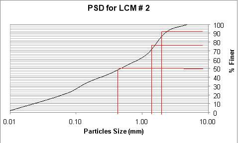
| mm | microns | |
| D(50) | 0.45 | 450 |
| D(75) | 1.65 | 1650 |
| D(90) | 2.6 | 2600 |
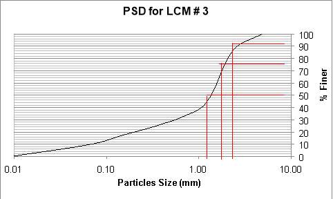
4.5.3 Test sample LCM #3 sieve analysis:
| Seive # | Seive Size (mm) | Empty Weight (g) | Weight after Shake (g) | Weight of retained Particles (g) | % Retained | Cumm. Retained % | % Finer |
| 4 | 4.75 | 750.9 | 751 | 0.1 | 0.2 | 0.2 | 99.8 |
| 8 | 2.36 | 444.3 | 450.7 | 6.4 | 12.8 | 13 | 87 |
| 16 | 1.18 | 634.3 | 656.2 | 21.9 | 43.8 | 56.8 | 43.2 |
| 30 | 0.60 | 601.6 | 607.7 | 6.1 | 12.2 | 69 | 31 |
| 40 | 0.43 | 334.7 | 336.6 | 1.9 | 3.8 | 72.8 | 27.2 |
| 50 | 0.30 | 535.9 | 537.7 | 1.8 | 3.6 | 76.4 | 23.6 |
| 100 | 0.15 | 508.2 | 511.3 | 3.1 | 6.2 | 82.6 | 17.4 |
| 200 | 0.08 | 489.5 | 492.9 | 3.4 | 6.8 | 89.4 | 10.6 |
| Pan | 0.01 | 473.4 | 478.5 | 5.1 | 10.2 | 99.6 | 0.4 |
| Sum (g) | 4822.6 | 49.8 |
| mm | microns | |
| D(50) | 1.3 | 1300 |
| D(75) | 1.8 | 1800 |
| D(90) | 2.8 | 2800 |
4.5.4 Test sample LCM #4 sieve analysis:
| Seive # | Seive Size (mm) | Empty Weight (g) | Weight after Shake (g) | Weight of retained Particles (g) | % Retained | Cumm. Retained % | % Finer |
| 4 | 4.75 | 750.9 | 750.9 | 0 | 0 | 0 | 100 |
| 8 | 2.36 | 444.3 | 449.4 | 5.1 | 10.2 | 10.2 | 89.8 |
| 16 | 1.18 | 634.3 | 651.4 | 17.1 | 34.2 | 44.4 | 55.6 |
| 30 | 0.60 | 601.6 | 610.2 | 8.6 | 17.2 | 61.6 | 38.4 |
| 40 | 0.43 | 334.7 | 338.7 | 4 | 8 | 69.6 | 30.4 |
| 50 | 0.30 | 535.9 | 539.8 | 3.9 | 7.8 | 77.4 | 22.6 |
| 100 | 0.15 | 508.2 | 514.5 | 6.3 | 12.6 | 90 | 10 |
| 200 | 0.08 | 489.5 | 492.9 | 3.4 | 6.8 | 96.8 | 3.2 |
| Pan | 0.01 | 473.4 | 474.5 | 1.1 | 2.2 | 99 | 1 |
| Sum (g) | 4822.3 | 49.5 |
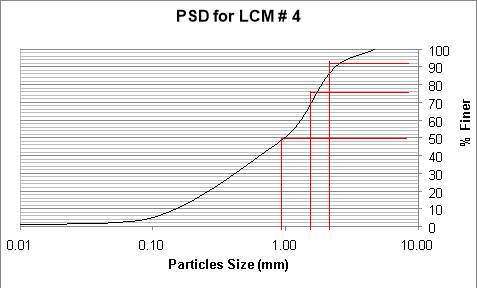
| mm | microns | |
| D(50) | 1 | 1000 |
| D(75) | 1.7 | 1700 |
| D(90) | 2.5 | 2500 |
4.5.5 Test sample LCM #5 sieve analysis:
| Seive # | Seive Size (mm) | Empty Weight (g) | Weight after Shake (g) | Weight of retained Particles (g) | % Retained | Cumm. Retained % | % Finer |
| 4 | 4.75 | 750.9 | 750.9 | 0 | 0 | 0 | 100 |
| 8 | 2.36 | 444.3 | 446.1 | 1.8 | 3.6 | 3.6 | 96.4 |
| 16 | 1.18 | 634.3 | 640.9 | 6.6 | 13.2 | 16.8 | 83.2 |
| 30 | 0.60 | 601.6 | 610.5 | 8.9 | 17.8 | 34.6 | 65.4 |
| 40 | 0.43 | 334.7 | 340.2 | 5.5 | 11 | 45.6 | 54.4 |
| 50 | 0.30 | 535.9 | 541.2 | 5.3 | 10.6 | 56.2 | 43.8 |
| 100 | 0.15 | 508.2 | 516.7 | 8.5 | 17 | 73.2 | 26.8 |
| 200 | 0.08 | 489.5 | 495.5 | 6 | 12 | 85.2 | 14.8 |
| Pan | 0.01 | 473.4 | 480.3 | 6.9 | 13.8 | 99 | 1 |
| Sum (g) | 4822.3 | 49.5 |
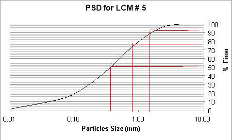
| mm | microns | |
| D(50) | 0.4 | 400 |
| D(75) | 0.9 | 900 |
| D(90) | 1.7 | 1700 |
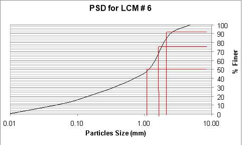
4.5.6 Test sample LCM #6 sieve analysis:
| Seive # | Seive Size (mm) | Empty Weight (g) | Weight after Shake (g) | Weight of retained Particles (g) | % Retained | Cumm. Retained % | % Finer |
| 4 | 4.75 | 750.9 | 750.9 | 0 | 0 | 0 | 100 |
| 8 | 2.36 | 444.3 | 449.7 | 5.4 | 10.8 | 10.8 | 89.2 |
| 16 | 1.18 | 634.3 | 653.6 | 19.3 | 38.6 | 49.4 | 50.6 |
| 30 | 0.60 | 601.6 | 608.2 | 6.6 | 13.2 | 62.6 | 37.4 |
| 40 | 0.43 | 334.7 | 337.1 | 2.4 | 4.8 | 67.4 | 32.6 |
| 50 | 0.30 | 535.9 | 538.2 | 2.3 | 4.6 | 72 | 28 |
| 100 | 0.15 | 508.2 | 512 | 3.8 | 7.6 | 79.6 | 20.4 |
| 200 | 0.08 | 489.5 | 493.1 | 3.6 | 7.2 | 86.8 | 13.2 |
| Pan | 0.01 | 473.4 | 479.8 | 6.4 | 12.8 | 99.6 | 0.4 |
| Sum (g) | 4822.6 | 49.8 |
| mm | microns | |
| D(50) | 1.2 | 1200 |
| D(75) | 1.9 | 1900 |
| D(90) | 2.5 | 2500 |
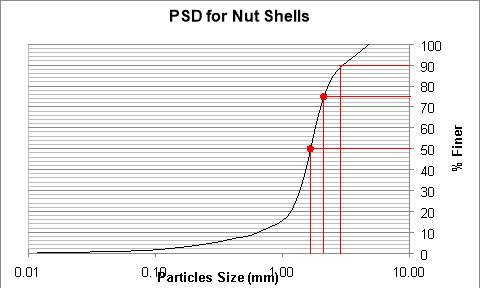
4.5.7 Nut Shells sieve analysis:
| Seive # | Seive Size (mm) | Empty Weight (g) | Weight after Shake (g) | Weight of retained Particles (g) | % Retained | Cumm. Retained % | % Finer |
| 4 | 4.75 | 750.9 | 750.9 | 0 | 0 | 0 | 100 |
| 8 | 2.36 | 444.3 | 453.2 | 8.9 | 17.8 | 17.8 | 82.2 |
| 16 | 1.18 | 634.3 | 665.1 | 30.8 | 61.6 | 79.4 | 20.6 |
| 30 | 0.60 | 601.6 | 607.3 | 5.7 | 11.4 | 90.8 | 9.2 |
| 40 | 0.43 | 334.7 | 335.7 | 1 | 2 | 92.8 | 7.2 |
| 50 | 0.30 | 535.9 | 536.9 | 1 | 2 | 94.8 | 5.2 |
| 100 | 0.15 | 508.2 | 509.5 | 1.3 | 2.6 | 97.4 | 2.6 |
| 200 | 0.08 | 489.5 | 490.2 | 0.7 | 1.4 | 98.8 | 1.2 |
| Pan | 0.01 | 473.4 | 474 | 0.6 | 1.2 | 100 | 0 |
| Sum (g) | 4822.8 | 50 |

| mm | microns | |
| D(50) | 1.7 | 1700 |
| D(75) | 2.1 | 2100 |
| D(90) | 2.9 | 2900 |
4.5.8 Fluid loss at 15ppb concentration for all blends
4.5.9 Fluid loss at 50ppb concentration for all blends
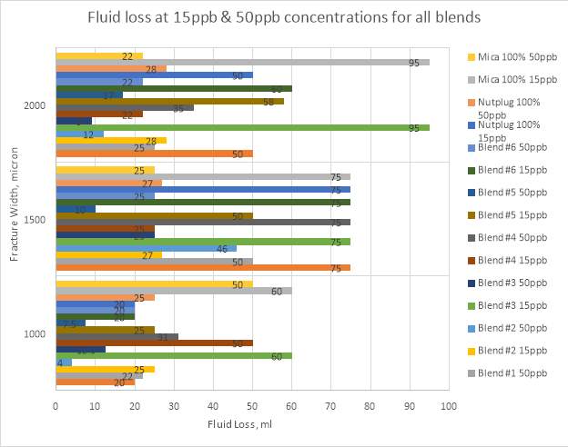
4.5.10 Fluid loss at 15ppb & 50ppb concentrations for all blends
4.5.11 Effect of fracture widths on fluid loss for all blends
5. Discussions
5.1 Effect of concentration in fluid loss
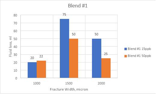
- Blend #1: Increasing concentration slightly affected the fluid loss in a negative way for the fracture width 1000 microns. However, for the larger fracture widths, the losses were reduced.
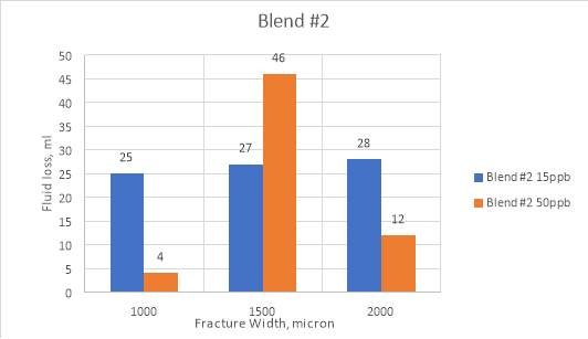
- Blend #2:Increasing the concentration for this blend reduced the fluid losses for the fracture width 1000 microns and 2000 microns. However, the opposite trend was observed for the fracture width of 1500 microns in the 50ppb concentration
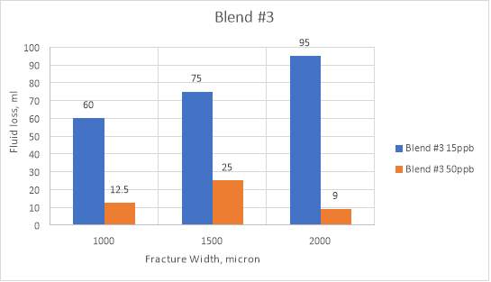
- Blend #3: The Increase in concentration decreased the fluid loss in all of the fracture widths.
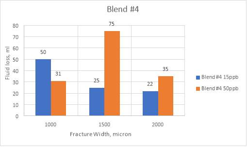
- Blend #4: Increase in concentration for the fracture width 1000 microns affected the fluid loss positively. However, for the fracture widths 1500 microns and 2000 microns, the fluid loss increased.
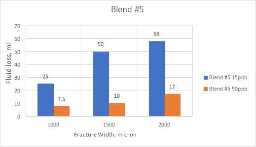
- Blend #5: The Increase in concentration affected the fluid loss positively in all the fracture widths.
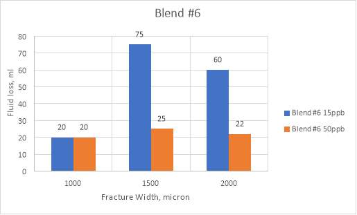
- Blend #6: The increase in concentration didn’t influence the fluid loss for the fracture width 1000 microns. However, the fluid loss decreased significantly for the fracture width 1500 microns & decreased slightly for the fracture width 2000 microns.
- NS 100%:The higher the concentration for the larger fracture widths, the better the results. However, the lower concentration for the small fracture width showed better results.
- Mica 100%:The higher the concentration leads to better sealing/lower fluid losses in all fracture widths.
5.2 PSD Analysis observation
Blend #1:
1000 microns
D50: 50% of the particles are larger 280 microns. However, it doesn’t satisfy the criteria.
D90: 10% of the particles are larger than 2600 microns. It satisfies the criteria.
1500 microns
D50: 50% of the particles are larger 280 microns. However, it doesn’t satisfy the criteria.
D90: 10% of the particles are larger than 2600 microns. It satisfies the criteria.
2000 microns
D50: 50% of the particles are larger 280 microns. However, it doesn’t satisfy the criteria.
D90: 10% of the particles are larger than 2600 microns. It satisfies the criteria.
Blend #2:
1000 microns
D50: 50% of the particles are larger 450 microns. It satisfies the criteria.
D90: 10% of the particles are larger than 2600 microns. It satisfies the criteria.
1500 microns
D50: 50% of the particles are larger 450 microns. It satisfies the criteria.
D90: 10% of the particles are larger than 2600 microns. It satisfies the criteria.
2000 microns
D50: 50% of the particles are larger 450 microns. However, it doesn’t satisfy the criteria.
D90: 10% of the particles are larger than 2600 microns. It satisfies the criteria.
Blend #3:
1000 microns
D50: 50% of the particles are larger 1300 microns. It satisfies the criteria.
D90: 10% of the particles are larger than 2800 microns. It satisfies the criteria.
1500 microns
D50: 50% of the particles are larger 1300 microns. It satisfies the criteria.
D90: 10% of the particles are larger than 2800 microns. It satisfies the criteria.
2000 microns
D50: 50% of the particles are larger 1300 microns. It satisfies the criteria.
D90: 10% of the particles are larger than 2800 microns. It satisfies the criteria.
Blend #4:
1000 microns
D50: 50% of the particles are larger 1000 microns. It satisfies the criteria.
D90: 10% of the particles are larger than 2500 microns. It satisfies the criteria.
1500 microns
D50: 50% of the particles are larger 1000 microns. It satisfies the criteria.
D90: 10% of the particles are larger than 2500 microns. It satisfies the criteria.
2000 microns
D50: 50% of the particles are larger 1000 microns. It satisfies the criteria.
D90: 10% of the particles are larger than 2500 microns. It satisfies the criteria.
Blend #5:
1000 microns
D50: 50% of the particles are larger 400 microns. It satisfies the criteria.
D90: 10% of the particles are larger than 1700 microns. It satisfies the criteria.
1500 microns
D50: 50% of the particles are larger 400 microns. However, it doesn’t satisfy the criteria.
D90: 10% of the particles are larger than 1700 microns. However, it doesn’t satisfy the criteria.
2000 microns
D50: 50% of the particles are larger 400 microns. However, it doesn’t satisfy the criteria.
D90: 10% of the particles are larger than 1700 microns. However, it doesn’t satisfy the criteria.
Blend #6:
1000 microns
D50: 50% of the particles are larger 1200 microns. It satisfies the criteria.
D90: 10% of the particles are larger than 2500 mic. It satisfies the criteria.
1500 microns
D50: 50% of the particles are larger 1200 microns. It satisfies the criteria.
D90: 10% of the particles are larger than 2500 mic. It satisfies the criteria.
2000 microns
D50: 50% of the particles are larger 1200 microns. It satisfies the criteria.
D90: 10% of the particles are larger than 2500 mic. It satisfies the criteria.
6. Conclusion and Recommendations
7. References
Advances in Petroleum Exploration and Development. (2011, June 30th).
Alsaba, M. T. (2015). Investigation of lost circulation materials impact on fracture gradient. Doctoral Dissertations. Retrieved from http://scholarsmine.mst.edu/doctoral_dissertations/2437
FANN Testing Equipment. (n.d.). Retrieved from Global Drilling Products & Services: http://www.globaldrilling-s.com/en/products/fann-laboratory-equipment/drilling-fluids-testing/filtration-hpht.html
GEORGE C. HOWARD AND P. P. SCOTT, J. (1951). AN ANALYSIS AND THE CONTROL OF LOST CIRCULATION. T.P. 3096.
GEORGE C. HOWARD and P. P. SCOTT, J. (April 12,1951). AN ANALYSIS AND THE CONTROL OF LOST CIRCULATION. SPE 941171.
IADC Drilling Manual. (2014).
Lavrov, A. (2016). Lost Circulation. Mechanisms and Solutions, Chapter 1 (1-11).
OFITE. (n.d.). Retrieved from OFI Testing Equipments: http://www.ofite.com/products/product/560-filter-press-low-pressure-bench-mount-with-co2-pressure-assembly
S.A.), A. N. (1999). An Overview of Air/Gas/Foam Drilling in Brazil. SPE-56865-PA.
Spears & associates. (2004). Oil field market report. Oklahoma: Spears & associates. Retrieved from https://spearsresearch.com/
Cite This Work
To export a reference to this article please select a referencing stye below:
Related Services
View all


Related Content
All TagsContent relating to: "Sciences"
Sciences covers multiple areas of science, including Biology, Chemistry, Physics, and many other disciplines.
Related Articles

DMCA / Removal Request
If you are the original writer of this dissertation and no longer wish to have your work published on the UKDiss.com website then please: