Energy Technology for Improved Efficiency in Commercial Buildings
Info: 30370 words (121 pages) Dissertation
Published: 9th Jun 2021
Tagged: ArchitectureEnergy
Advanced co-generation systems with organic Rankine cycle in commercial buildings
Abstract
Commercial and industrial buildings have high energy demand profiles; hence it has become vital to find more efficient ways of supplying energy to these sectors, both for the good of reducing emissions and for companies to reduce cost. CHPQA is one policy that can make the generator exempt from carbon taxes, making it more attractive for companies to incorporate CHP’s. This project was undertaken to design a model and evaluate the interaction and performance of one cogeneration combination, a CHP-ORC configuration. The ICE is one of the most common types of prime movers for CHP’s below 1 MW capacity and was chosen because of its reliability, cost, dispatchability and maturity of technology. Most of industrial application of ORC systems is geothermal in nature and ORC types associated with geothermal application are not considered. This leaves sub-critical and supercritical ORC systems, but simplicity is preferred and hence a sub-critical ORC system is selected. In terms of simplicity, tube-in-tube is simplest and is used for further simulation. For the ORC, the selection of the WF is vital to produce an optimally performing system and five were chosen for further examination, Toluene, R1233ZD, R1234ZE, P-Xylene and Benzene.
The model was used to validate against engines available in the market for CHP-1520, CHP-502 and CHP-310. The results were found to be in good agreement with industrial data and were within tolerances specified in the data sheet. Two ORC models were used for this thesis, one for a simple ORC system and one to include a recuperator. Toluene, R1233ZD and Benzene were found to be the three most suitable fluids for both simple and recuperated systems. The variation between the two systems are significant. There is a huge benefit of incorporating a recuperator with consistently higher performance and lower cost. R1233ZD sees the highest increase in power and efficiency as it is the only fluid that has significant degree of superheating. For Toluene, the total evaporator size is highest for the simple system. By incorporating a recuperator, 70% of evaporator area could be cut. For R1233ZD and Benzene, the area saving is not as high as Toluene, but still significant, saving 47% and 27% respectively. The results of this study indicate that the efficiency increased when operating at part load, because the temperature increase of the exhaust gas played a larger role than the decrease in exhaust mass flow rate.
Of the three fluids, Benzene is the cheapest for both systems. The most expensive is Toluene, while R1233ZD lies in the middle of the SIC range. The cost savings from incorporating a recuperator is the most beneficial for Toluene and lowest for Benzene. The main weakness with the methodology is not accounting for fluid cost. Toluene and Benzene have similar cost, but there is a lack of data for R1233ZD costs. R1233ZD is a relatively new fluid and can be determined to be more expensive and it is possible that R1233ZD shifts to be more expensive than Toluene overall.
A limitation of this study is that the behaviour found from the modelling will be applicable to ICE CHP, sub-critical ORC, tube-in-tube HEX and pumps with flat characteristic curves only. Despite the limited application, this study manages to give a framework and will be able to expand the technology base in the future. Additionally, it is suggested that the pump and expander to be included in future work to give the full picture of part load performance.
Table of Contents
2.1. CHP technologies and applications
2.1.1. Thermodynamic modelling of CHP
2.2. ORC technology and applications
2.2.1. Thermodynamic modelling of ORC
2.2.2. Working fluid selection
2.3. Integration of cogeneration systems
3.2. Simple ORC system optimization and model
3.3. Recuperative ORC system optimization and model
3.4. Heat exchanger sizing and part load optimisation
3.5. ORC module costing technique
Chapter 4. Results and discussion
4.2. Analysis of optimized ORC system results
4.3. Heat exchanger sizing results and analysis
4.4. Part load performance of the simple and recuperated ORC system
4.4.1. The influence of the HEX on the ORC system
4.4.2. Comparison of overall heat transfer coefficient
4.4.3. Influence of other ORC components
List of Figures
Figure 1 Electricity demand profile for a winters day in the UK………………………..
Figure 2 Energy demand with store size. Energy demand per unit area decreases with increased store size…..
Figure 3 CHP-ICE system configuration……………………………………….
Figure 4 Four stroke engine cycle…………………………………………..
Figure 5 ORC schematic…………………………………………………
Figure 6 T-s diagram of a non-recuperative ORC cycle……………………………..
Figure 7 CHP-ORC system configuration………………………………………
Figure 8 T-s diagram of a simple ORC cycle repeated………………………………
Figure 9 (a) ORC system with recuperator schematic (b) T-s diagram of system……………..
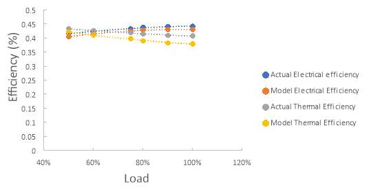
Figure 10 Part load efficiency comparison for CHP- 1520 kW…………………………
Figure 11 Part Load efficiency comparison CHP- 502 kW……………………………
Figure 12 Part load efficiency comparison CHP-310 kW…………………………….
Figure 13 Part load power comparison CHP-1520 kW………………………………
Figure 14 Part load power comparison CHP-502 kW……………………………….
Figure 15 Part load power comparison CHP-310 kW……………………………….
Figure 16 Exhaust mass flow part load comparison CHP-1520 kW………………………
Figure 17 Exhaust flow part load comparison CHP-502 kW…………………………..
Figure 18 Exhaust flow part load comparison CHP-310 kW…………………………..
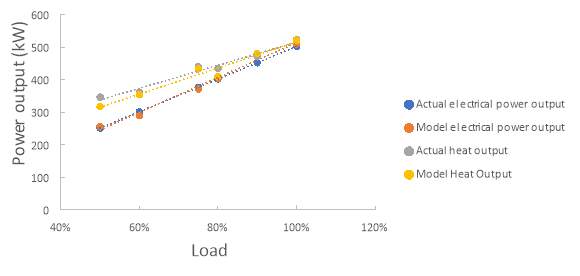
Figure 19 Exhaust and cooling circuit output comparison CHP-1520 kW………………….
Figure 20 Exhaust and cooling circuit output comparison CHP-502 kW…………………..
Figure 21 Exhaust and cooling circuit output comparison CHP-310 kW…………………..
Figure 22 Optimised flow rates comparison with CHP load (CHP-1520 kW, ORC with recuperator)…
Figure 23 Evaporator area optimised against CHP load comparison (CHP-1520 kW)…………..
Figure 24 Evaporator area optimised against CHP load comparison (CHP-1520 kW, ORC with recuperator)…..
Figure 25 Condenser area optimised against CHP load comparison (CHP-1520 kW)…………..
Figure 26 Condenser area optimised against CHP load comparison (CHP-1520 kW, ORC with recuperator)…..
Figure 27 Recuperator area comparison (CHP-1520 kW)……………………………
Figure 28 Simple ORC system comparing part load performance of different WF optimised against 100% CHP-1520kW load…..
Figure 29 Recuperated ORC system comparing part load performance of different WF optimised against 100% CHP-1520kW load…..
Figure 30 Overall heat transfer coefficient of the evaporator for simple ORC system………….
Figure 31 Overall heat transfer coefficient of the evaporator for recuperated ORC system………
Figure 32 ORC efficiency against heat source temperature collected from industrial data [80]……
Figure 33 Pump characteristic curve…………………………………………
Figure 34 Radial turbine performance map…………………………………….
Figure 35 Specific investment cost of simple ORC system……………………………
Figure 36 Specific investment cost of recuperated ORC system………………………..
Figure 37 TSO model flow chart process………………………………………
List of Tables
Table 1 Advantages and disadvantages of prime movers……………………………
Table 2 Cost breakdown of ICE CHP Unit………………………………………
Table 3 Review of different ORC architectures…………………………………..
Table 4 Working fluid selection…………………………………………….
Table 5 Review of HEX type used in ORC system literature…………………………..
Table 6 Model constants and limits………………………………………….
Table 7 Cost coefficients for cost correlation equations…………………………….
Table 8 Conversion table for currency and inflation……………………………….
Table 9 Optimised ORC system values for the simple ORC cycle (For CHP-1520 kW)…………..
Table 10 Optimised ORC system values for recuperated ORC cycle (For CHP-1520 kW)………..
Table 11 Optimised ORC system values for the simple ORC cycle (CHP-502 kW)……………..
Table 12 Optimised ORC system values for recuperated ORC cycle (CHP-502 kW)……………
Table 13 Optimised ORC system values for the simple ORC cycle (CHP-310 kW)……………..
Table 14 Optimised ORC system values for recuperated ORC cycle (CHP-310 kW)……………
Table 15 LMTD for simple ORC system……………………………………….
Table 16 LMTD for recuperated ORC system……………………………………
Abbreviations
| CHP Combined Heat and Power | SI Spark Ignition |
| CHPQA Combined Heat and Power Quality Assurance | CI Compression Ignition |
| ICE Internal Combustion Engine | HEX Heat Exchanger |
| WF Working Fluid | TDC Top Dead Centre |
| HFC Hydrofluorocarbons | BDC Bottom Dead Centre |
| COP Coefficient of Performance | ORC Organic Rankine Cycle |
| EPC Electricity Production Cost | ODP Ozone Depletion Potential |
| TSO Technology selection and operation | GHG Green House Gas |
| SIC Specific Investment Cost | OFC Organic Flash Cycle |
| OTEC Ocean Thermal Energy Conversion | HFO Hydrofluoroolefins |
| NOX Nitrogen Oxides | CFD Computational Fluid Dynamics |
| LMTD Logarithmic Mean Temperature Difference | GWP Global Warming Potential |
| GPM Gallon per minute | kW KiloWatt |
| HP Horsepower | SHD Superheating degree |
| DIPPR Design Institute for Physical Properties | HFO Hydrofluoroolefins |
| HCFO Hydrochloroflouroolefin | SIC Specific Investment Cost |
| CEPCI Chemical Engineering Plant Cost Index | bTDC before Top Dead Centre |
| AFR Air to Fuel Ratio | LHV Lower Heating Value |
Nomenclature
| A Area (m2) | Subscripts |
| b Bore (m) | comp Compressor |
| CD
Valve discharge coefficient (-) |
cyl Cylinder |
| cp
Specific heat capacity (kJ/kg K) |
cw Condenser water |
| Cp0
Cost ($) |
dis Displacement |
| D Diameter (m) | ex Exhaust |
| f Friction coefficient (-) | exp Expander |
| h Specific enthalpy (kJ/kg K) | g Gas |
| hg
Heat transfer coefficient (W/m2 K) |
g,el Electric generator |
| k Thermal conductivity (W/m K) | hs Heat source |
| l
Crankshaft rod length (m) |
Intake Intake |
| L Pipe length (m) | Net Net |
| ṁ
Mass flow rate (kg/s) |
p Piston |
| Nu Nusselt number (-) | ref Refrigerant |
| P
Pressure (kPa) |
v Valve |
| Pcrit
Refrigerant critical pressure (kPa) |
w Wall |
| Pm
Motoring pressure (kPa) |
wf Working Fluid |
| PP Pinch Point (K) | 0 Initial conditions |
| Pr Prandtl number (-) | 1,2,3,4,5,6,7,8,9 State |
| q Heat load (kW) | i/o inlet/outlet |
| Qcond
Condenser heat load (kW) |
Is Isentropic |
| Qevap
Evaporator heat load (kW) |
Drop Drop |
| Qin
Combustion heat input (kJ) |
Max Max |
| Qw
Heat losses through wall (kJ) |
|
| R Gas constant (kJ/kg K) | |
| Re Reynolds Number (-) | |
| r Volume ratio (-) | |
| rps Revolution per second (rad/s) | |
| SHD SuperHeating Degree (-) | |
| T Temperature (K) | |
| u Velocity (m/s) | |
| U Overall heat transfer coefficient (W/m2 K) | |
| UP
Piston velocity (m/s) |
|
| V Volume (m3) | |
| Ẇ
Work (kW) |
|
| xb
Wiebe function (-) |
|
| y Instantaneous length (m) | |
| Greek symbols | |
| Κ Kinematic viscosity (m2/s) | α Wiebe constant |
| ν
Volume flow rate (L/s) |
∆
Difference |
| η Efficiency (-) | ρ Density (kg/m3) |
| µ Dynamic viscosity (Pa s) | γ
Ratio of specific heats (-) |
| ε Effectiveness (-) | ϑ
Crankshaft angle (deg) |
| π pi mathematical constant (-) | ω
Rotational speed (rad/s) |
Chapter 1. Introduction
1.1. Motivation
Commercial and industrial buildings have high energy demand profiles; hence it has become vital to find more efficient ways of supplying energy to these sectors, both for the good of reducing emissions and for companies to reduce cost [1]. There has been an uptake in CHP units for the commercial sector [2], however, in many cases electricity has a higher demand than heat. The abundance of heat from CHPs are in order of magnitude higher, so there has been an interest in connecting CHP units to ORC for additional electricity generation. There are also policies in place to make CHPs an attractive option. CHPQA is one such policy which applies to CHPs that is categorised as good quality, meaning it needs to be able to save a certain amount of primary energy and efficiencies depending on capacity. This can make the generator exempt from carbon taxes and other fees as described in Ref. [3]. To determine the suitability, it is required to see which is the most efficient, gives minimal emissions and cost associated with the technologies. This thesis reviews CHP and ORC systems and from this review models selected technologies to determine the performance of the CHP-ORC configuration.
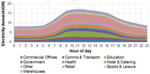
Figure 1 Electricity demand profile for a winters day in the UK [4] |
Figure 1 illustrates the electricity demand profiles of different service sectors on an average winters day and every sector follows this electricity profile as can be observed [4]. There are seasonal variations that can give insightful information, but more importantly that electricity and heat demand is highest during winter seasons and lowest during summer and opposite for cooling. Additionally, demand is highly variable from building to building within the same sector, depending on location, size, inventory and architecture. For this reason, it is better to suggest an optimal capacity range of the coupled CHP-ORC unit with the demand range of a specific building. As every sector have their own criteria to meet energy demand it is important to choose one sector to focus on. In this thesis the focus is on supermarket retailers as they use 3.5% of the electricity and accounts for 1% of all GHG emissions in the UK [5]. Hence, there is an opportunity to decarbonise this sector and to find the most suitable solutions for it. Figure 2 show energy requirements depends on store size, with larger store sizes using energy more efficiently. The aims and objectives of the thesis will now be presented.
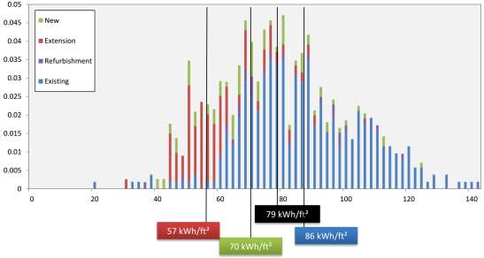
Figure 2 Energy demand with store size. Energy demand per unit area decreases with increased store size [5] |
1.2.  Aim
Aim
The aim of the project is to evaluate the performance characteristics and specific investment cost in coupling an ORC system with a CHP unit that can be used further in the decarbonisation of a large supermarket retailer in the UK.
1.3. Objectives
To achieve the aim, key objectives are:
- Review of CHP and ORC system technology, in addition to economic considerations for commercial building application.
- Identify first principle modelling methods for CHP and ORC systems for accurate analysis of performance in Matlab.
- Review CHP-ORC integration technology and modelling methods.
- Incorporate a recuperator to the ORC model to determine its benefits.
- Model the CHP-ORC system to represent the part load performance of the CHP-ORC system. These results will lay the foundation for a thermo-economic analysis
1.4. Structure of thesis
To determine the suitability of technologies, it is required to determine the best performing in terms of efficiency, emission and cost. In this thesis, a technology review of CHP and ORC system will be discussed in chapter 2. Within this section the thermodynamic modelling methods, costing, system integration methods of these technologies will also be presented. Chapter 3 details the methodology used in modelling the different systems or using correlations in the case of costing ORC systems. Chapter 4 will present and analyse the results of the models. Chapter 5 concludes the thesis with recommendations on future work.
Chapter 2. Literature review
2.1. CHP technologies and applications
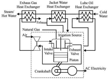
The principle of CHP is simultaneously generating electricity and heat to meet the respective demands. Heat always accompany any energy production as a by-product, in accordance with 2nd law of thermodynamics, hence extracting the heat will raise the overall efficiency of the unit. This allows reductions in emissions due to the reduction of fuel usage. CHP has found application in both domestic and non-domestic settings, where for non-domestic buildings, hospitals, data centres, supermarkets, malls and schools have experience in the technology. Whether priorities are cost considerations for supermarkets, malls or schools, alleviating cost during peaks of demand, or security of supply for hospitals and data centres, CHP is an effective technology to fulfil different criteria [6]. Figure 3 show a standard CHP unit with an ICE prime mover.
|
Supermarket retailers have a higher demand for electricity due to refrigeration, which accounts for about 20-60% of energy consumption, while heat accounts for on average about 10% of electricity demand [7]. By using the heat by coupling with an ORC unit for electricity, demand can be met more efficiently [8]. The main consideration to make for CHP selection is the prime mover. Criteria for selecting prime mover for supermarkets is related to the unit size, dispatchability, reliability, flexibility and cost considerations. Table 1 shows a review of prime movers with advantages and disadvantages.
Table 1 Advantages and disadvantages of prime movers [9]
| Prime Mover | Steam Turbines | Gas Turbines | ICE | Stirling Engines | Fuel Cells |
| Advantages | Long life cycle | Low initial cost | Rapid start | Very quiet and low emissions | Low O&M cost and environmental impact |
| High overall efficiency | High availability and efficiency at larger size | High availability and low first cost | Independent electricity and heat production | Quiet operation and flexible fuel choice | |
| Flexible steam extraction | Fast manufacturing and installation | Efficiency less sensitive to load variation than gas turbine | Fuel independent and long maintenance intervals | High efficiency over load range and modularity | |
| Disadvantages | Bulky construction | Output and efficiency depend on ambient temperature | Relatively high noise and emissions | Limited availability | High capital cost because it is under development |
| Slow start-up and response to load fluctuation | High noise level and lower mechanical efficiency than ICE | Regular maintenance with high maintenance cost | Expensive materials for hot part of engine | Limited variability and poor ability for multiple starts | |
| High initial cost | Poor efficiency at low load | Require cooling and waste heat is split | Need further development | Lack of field data in O&M and contaminant sensitive | |
| Capacity | Up to 250 MW | Up to 250 MW | Up to 75 MW | Up to 55 kW | Up to 2 MW |
| Electrical efficiency | 15-38% | 18-36% | 25-45% | 15-35% | 37-60% |
| Overall efficiency | 80% | 65-75% | 65-80% | 60-80% | 55-80% |
| Waste Heat temperature | Up to 100 | 120-350 | 80-200 | Up to 85 | Up to 1000 |
| Part Load Efficiency | Moderate | Low | High | Moderate | Very High |
| Start-up time | >1h | >10min | >10s | – | >3h |
| Fuels Used | Natural gas and bio-fuels | Propane, natural gas, distillate oil, biogas | Diesel, natural gas, propane | Natural gas and biofuels | Hydrogen, methanol, natural gas |
| Lifetime(h) | 30000-50000 | 5000-40000 | 20000-50000 | 10000-30000 | 10000-65000 |
Of these technologies, ICE is the most common for capacities below 1MW with maturity of the technology the main reason [9]. Steam turbines have slow response due to large temperature operating ranges so there is inertia involved. It is large in size with high cost and mainly used for steam power plants making it unfeasible for supermarket use. Gas turbines are like ICEs, but is more sensitive to load variation and is better applied to settings which require higher capacity. Both Stirling engines and fuel cells have very compelling advantages, but are limited due to being in the initial stages of development, hence expensive. ICE is hence the prime mover of choice for supermarket application. First, the technology is mature and comparatively cheap, giving maximum returns for the investment. Second, its performance is relatively constant with load of the engine above 30% load [10], making it very flexible to meet demand. Finally, it can respond quickly to start-up and changes in load. To be able to respond quickly is important to adapt to changing load throughout the day. ICE offers the best balance of specifications for use in supermarkets, which is why it is the main choice for use in this thesis [8].
2.1.1. Thermodynamic modelling of CHP
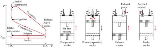
There are many models of ICE CHP that has been derived, but it is the method used in Ref. [11] using Matlab software for modelling purposes that will be modified to fit the purpose of the thesis. The model is a dynamic lumped model that uses energy and mass balance to predict the SI engine operation and hence get an accurate model of the performance of the CHP model. The detailed model with equations will be explained in the methodology section. This section aims to explain the inner working of the spark ignition ICE. Figure 4 show how a four-stroke engine operates. It is important to define TDC (piston on top) giving minimum volume and BDC (piston on bottom) giving maximum volume of the cylinder.
|
An ICE following an Otto cycle goes through four processes. First, the compression stroke goes from BDC to TDC where the fuel and air has been blended to give a combustible mix and ignited by a spark plug. Following from this phase, the combustion occurs and the piston goes back to BDC transmitting the revolving energy to the generator to generate electricity. The final stroke moves the piston back to TDC, exhausting residual waste gas as waste heat and sent to evaporator of the ORC unit or generator of the AC, when the piston goes back to BDC, air-fuel mixture again enters the cylinder to close the cycle [12]. The ICE CHP system is modelled using first law principles, by solving mass flow and energy conservation equations for a control volume where the boundaries are denoted in Figure 4 for every position of the piston.
Although efficiencies are relatively constant past a certain load percentage, it can have a significant effect on the temperature output of the waste heat. It is difficult to match load performance between the CHP and ORC systems. Operating the CHP at full load does not necessarily mean the bottoming cycles will operate at full load and even if it does, part load performance variations will most likely not be synchronized. There are two efficiencies associated with a CHP, thermal efficiency and electric efficiency. It is important to distinguish between the two as they vary differently with load and in opposite directions, electric efficiency decreases with part load and opposite with thermal efficiency. The reason for this will be explained later, but this is something an ORC system can take advantage of when coupled with CHP’s as it is driven by the heat supplied by the CHP. However, the use of constant efficiency curves or empirically derived efficiency curves comes short where selection and design of components are concerned [13]. To make the model self-contained it is assumed constant specific heat for exhaust gas, exhaust gas not cooled below dewpoint and waste heat defined as remaining non-converted fuel energy.
2.1.2. CHP costing
Table 2 show the cost of installing an ICE CHP per kW. It can be observed that with increasing capacity it becomes cheaper per kW, this is because of economies of scale. The data on breakdowns and specific investment cost of CHP’s are widely available compared to ORC systems. Hence, there will be no further focus on the costing of CHP’s.
Table 2 Cost breakdown of ICE CHP Unit [16-17]
|
Capital cost $/kW |
|
|
System
|
|
|
| 1 | 2 | 3 | 4 | 5 | |
| Nominal Capacity (kW) | 100 | 633 | 1121 | 3326 | 9341 |
| Equipment (Costs in 2013 ($/kW) | |||||
| Generator set package ($) | 1400 | 400 | 375 | 350 | 575 |
| Heat recovery ($) | 250 | 500 | 500 | 500 | 175 |
| Interconnect ($) | 250 | 140 | 100 | 60 | 25 |
| Exhaust gas treatment ($) | 750 | 500 | 230 | 150 | |
| Total Equipment ($) | 1900 | 1790 | 1475 | 1140 | 925 |
| Labour/Materials ($) | 500 | 448 | 369 | 285 | 231 |
| Total Process Capital ($) | 2400 | 2238 | 1844 | 1425 | 1156 |
| Project and construction management ($) | 125 | 269 | 221 | 171 | 139 |
| Engineering fees ($) | 250 | 200 | 175 | 70 | 30 |
| Project Contingency ($) | 95 | 90 | 74 | 57 | 46 |
| Project Financing ($) | 30 | 42 | 52 | 78 | 62 |
| Total Plant Cost ($/kW) | 2900 | 2837 | 2366 | 1801 | 1433 |
2.2. ORC technology and applications
The fundamental cycle is the Rankine cycle undergoing a two phase transition between a liquid and gaseous state for steam to produce electricity [12]. An ORC system is analogous to the Rankine cycle, but instead of using steam as the WF, it is an organic fluid selected to suit the lower temperature ranges. The source of heat is flexible, the main applications being geothermal wells, solar, OTEC and CHP as the temperature range is lower. The ORC system have an upper temperature limit of about 450 °C where efficiency drops significantly [16]. Figure 5 shows a schematic showing the ORC system.
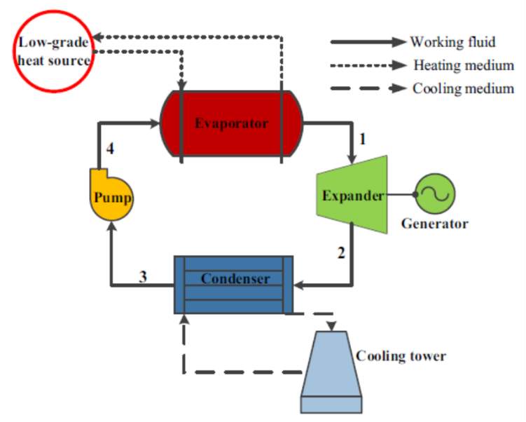
|
Table 3 compares 4 types of ORC configurations available. The sub-critical cycle is the basic ORC cycle, having a single stage expander and is cheap. Even with relatively low efficiency sub-critical cycle is the easiest to model with least amount of computer resource required, which is why sub-critical is the cycle of choice for this thesis. OFC uses geothermal brine as WF and is hence not applicable for supermarkets. Both trilateral and supercritical cycles are more complex hence expensive computational wise. There is additional modifications available such as regenerators and recuperators. Recuperators will be added in the modelling to compare the benefits between a simple sub-critical ORC system and a recuperated system.
Table 3 Review of different ORC architectures
| Sub-critical cycle [17] | Supercritical cycle [18] | Trilateral cycle [19] | Organic flash cycle (Geothermal application) [19] |
| Advantages | |||
| Simple design with less components hence cheaper | Better thermal match between heat source and WF | Boiling avoided, shifting pinch point limitation | Good temperature profile match between heat carrier and WF |
| Single stage expander | No pinch limit [20] | Higher potential to recover heat, better efficiency | Can be more efficient, but requires substantial modifications |
| Superheating not required with isentropic or dry fluids, although depending on latent heat of the fluid, superheating might occur. | Does not go through two phase transitions hence less irreversibility | Good temperature profile match between heat carrier and WF | |
| Disadvantages | |||
| Relatively low efficiency | Higher pressures required adding safety concerns | Require two-phase expander with high isentropic efficiency | Many extra components needed hence more expensive |
| Large HEX requirements for best extraction | Complexity | High moisture content at expander exit.
Reduces efficiency and requires turbine blade reinforcement, increases cost |
|
Using an ORC system is reliable, has minimal maintenance, easy access to components and most importantly reliable performance. One major barrier for more widespread use is the availability of waste heat sources, but there is an opportunity with high grade heat from CHPs being extracted for further power generation [21]. The selection of appropriate components fit for application is vital to its performance where Ziviani [22] remarks that the expander being a bottleneck of performance if not selected appropriately, but selection of the expander is not an aim for this thesis.
2.2.1. Thermodynamic modelling of ORC
To get an accurate analysis of the ORC unit an appropriate modelling method needs to be selected. There are differences between modelling an ORC unit compared to ICE CHP, mainly because the CHP unit produces energy from a fuel source, while ORC recovers waste heat. The general operation of an ORC unit is described below.
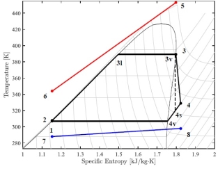
|
Figure 6 illustrates the whole ORC operation, starting at the evaporator as it receives waste heat from the CHP. Point 3v and 4v are saturated vapor, point 4 is superheated vapour, point 1 is saturated liquid, point 4s is the point reached if the expander was isentropic and point 2 is compressed liquid. The whole evaporator process is shown in Figure 6 (process 2-3). The evaporator of the ORC system is a HEX divided into three sections of a pre-heater, evaporator and superheater. The WF is sent to an expander, generating electricity (process 3-4). A wet fluid changes the dome slope on the right side to a negative one, isentropic a vertical line and a dry fluid positive slope. It is important in determining whether superheating is required to avoid droplet formation during expansion, as it can damage the expander blades because of the high speeds it operates [23]. Essentially, it is vital for state 4 to remain outside the dome, but is only a requirement for sub-critical ORCs. Following this process, the WF is sent further to the condenser for cooling (process 4-1). At the end of the cycle the WF is pumped back to evaporator pressure (process 1-2) to repeat the cycle. The ORC unit can receive a heat input from a variety of sources such as geothermal wells, solar and CHP. The CHP-ORC configuration is chosen because it is the most reliable source, as geothermal is geographically restricted and solar is intermittent. Energy analysis methods has seen much use in literature such as Ref. [21, 28–31] as using the fundamental laws of thermodynamics to perform the modelling is core to all models. The methods described are steady-state models. It is important to note that these methods are system level modelling methods and does not take into account the more detailed modelling such as CFD for HEXs as it is outside the scope of this thesis [27]. A system level method is more appropriate as more detailed modelling is hard to couple with other software as remarked by the authors of Ref. [28].
The pinch point analysis aims to minimise energy consumption at HEXs to fully utilise the waste heat. It is the minimum distance between the red external condition line and point 5 in Figure 6. The smaller the distance between these two points the larger the HEX is required to be, hence increasing investment cost and friction losses (longer pipes). The optimal pinch point is identified to be between 3-7 °C for best balance of economics and performance [25]. The pinch point method was invented to be able to design more efficient heat transfer pathways for HEX’s, reducing otherwise redundant area of heat exchangers. It is important to note that energy balance alone will not satisfy the desired outcome, but to achieve a balance between performance and economics using thermo-economic modelling [29].
In addition, there are methods to model off-design operating ranges, in fact, as most engineering solutions are usually designed for one specific condition, making off-design operation more common. For this thesis, the main focus is to determine how the heat exchanger influences the part load performance of the ORC system being driven by a CHP. There are then two considerations, one that first optimises the size of the ORC system design point power output and sizing of the HEX area. After optimising the size of the ORC system, parameters can be extracted to size the HEX area, which is achieved by combining the methods used by Chatzopolou [11, 33]. The part load performance of the ORC system influenced by the HEX’s can then be calculated.
2.2.2. Working fluid selection
Working fluids have been analysed under conditions varying from low to high temperature ORC system applications, though for this study the focus is on high temperature fluids. There are no fluids that fit into every role, which is why fluid selection is very important. Studies by Lai et al [31] analysed many different types of working fluids for high temperature application such as alkanes, aromates and siloxanes. It is found that a majority of present high-temperature ORC plants use Toluene [32] or siloxanes [33]. However, for siloxanes it is found to have rather low efficiency because of having low critical pressure characteristics [31] and hence not considered in this thesis. Drescher and Bruggeman [34] used a software to consider suitable WF for various heat source temperatures. Key criterions include cost, thermodynamic properties, safety and material interaction. With the DIPPR software, Drescher and Bruggeman [34] found alkylbenzene to have the highest efficiencies which Toluene falls under. Based on a literature survey by Rahbar et al [16], Benzene and Toluene fell under high temperature fluids. With these studies in mind, hydrocarbons were chosen based on the most promising thermodynamic properties and operating temperature ranges as can be seen in Table 4. Additionally, hydrocarbons are in the category of low GWP and ODP making them advantageous in their selection, although highly flammable. Keeping the system away from flammable sources and below auto-ignition temperature is vital, hence is showed in Table 4. As auto-ignition temperature is below heat source temperature, the hydrocarbons considered are appropriate.
The WF affects performance, depending on characteristics of the fluid and operational conditions of the ORC system. Parameters of importance for a WF include: wet, dry or isentropic fluid, latent heat of vaporisation, specific volume, corrosiveness, flammability and toxicity. Environmental factors such as ODP is required by law to be zero and GWP cannot exceed certain limits, depending on application, as specified by EU F-gas regulations [35]. There are old refrigerants still in use where GWP remain high, but is currently being phased out. To replace high GWP refrigerants in line with EU F-Gas regulations as stated in Ref. [36], new HFO refrigerants have been developed (e.g. by Honeywell) that have low GWP [37]. However, HFOs are still expensive compared to other commercial refrigerants and has yet to see widespread use. Some HFO refrigerants will still be considered to see the viability for future use. The hydrocarbons are readily available.
The fluids require good GWP, ODP, toxicity, corrosiveness and flammability characteristics, which all the WF’s in Table 4 have. Organic fluids are toxic by nature, so having low toxicity is optimal [38]. The refrigerants are notable as R1234ZE is the first type of WF under HFO and R1233ZD under HCFO. These refrigerants are the first of its kind that have zero ODP and very low GWP below 10. Lastly, toxicity needs to be minimal, as some organic fluids can be toxic. The organic fluids presented will have varying degrees of problems with prolonged inhalation in case of leakage, therefore good ventilation is required in most cases to prevent these issues. Although refrigerants are normally not applicable for high-temperature application, it is of interest to test these low ODP and GWP refrigerants for ORC system application to check for viability. R1233ZD is also used in the same model as Ref. [11].
Table 4 Working fluid selection
| Working Fluid | Temperature range (°C, evaporator) | Heat source temperature (°C) | Critical pressure (kPa) | Auto-Ignition temperature (°C) | Application | Reference |
| Toluene | 265-300 | 250-500 | 4109 | 530 | Waste heat recovery | [1-2] |
| R1234ZE | – | – | 3636 | 368 | Refrigerant for commercial refrigeration | [40] |
| p-Xylene | 327 | 327 | 3500 | 530 | Waste heat recovery | [1-2] |
| R1233ZD | – | – | 3573 | 380 | Refrigerant for chillers and R123 replacement | [11, 40] |
| Benzene | 67-287 | 100-470 | 4890 | 560 | Waste heat recovery | [39] |
The CHP-ORC coupling in this case is a high temperature application with the heat source being in the 350-450 °C range. A high temperature working fluid is required combined with required properties based on good flammability, GWP and ODP properties. It is crucial to keep operating temperature ranges lower than auto-ignition temperature. Although the heat source temperature is high, the actual operating temperature will be lower depending on HEX effectiveness and pinch point limits. All the fluids considered will have very low GWP and no ODP.
Table 4 shows working fluids considered with accompanying operating temperatures and desired thermal properties from various references. Some additional important parameters include critical pressure. If the maximum pressure of the ORC system does not exceed the critical pressure it will be at subcritical conditions. Superheating for dry and isentropic fluids is not desirable for a simple ORC system and increases irreversibility [42]. Superheating for dry and isentropic fluids will mean more heat will have to be wasted at the condenser. If a recuperator is incorporated some degree of superheating would be beneficial for efficiency as some of the heat can be used to raise the temperature on the liquid side, both reducing preheater area and increasing work output.
The working fluid selection was in the end based on a combination of the parameters in Table 4. The performance could not be determined by these values itself and these WF’s were chosen to be run through an ORC optimizer. Of the alkylbenzenes, Butylbenzene was found to be the most efficient, but as REFPROP does not support this fluid, Benzene is chosen. From these initial five, it will be narrowed down to three depending on the highest output and efficiency as a result from the optimizer.
2.2.3. ORC costing
Unlike CHP’s, there is a lack of commercial data available regarding ORC costing and hence a cost correlation for each component is used, where the same equations are used for some components, but with differing constants. The components in question are the pump, pump motor, expander, evaporator/condenser and preheater/desuperheater. The costing correlation is presented by Turton et al. [43] for expanders and Seider et al. [44] for the rest of the components. As these correlations are based on figures at the time they were written and US dollar as currency as result, various conversions are required to account for inflation/deflation for present values using CEPCI values and currency conversions. The correlation and conversion factors will be presented in the economic analysis of the methodology section.
2.3. Integration of cogeneration systems
In this section, the integration of the system is discussed. It will be separated into two sections, one for CHP-ORC configuration and one for HEX waste heat recovery units. A review on integration methods maximising performance will be presented, as well as how to optimise HEXs and choosing the HEX in accordance with what literature have used the most.
A cogeneration system needs to balance supply with demand required from the supermarket, but there is a certain amount of complexity here. As the waste heat from the exhaust of the CHP is sent to the HEX that couples the CHP and ORC system to supply power, means that the ICE CHP unit can deliver less power because some of the demand will be fulfilled by the ORC system. This in turn changes the dynamics, potentially shifting the performance of the system. The ICE CHP unit with its lower load, supply waste heat of higher temperature than originally anticipated. This interaction is important to capture and predict to operate optimally. Following this, it is important to derive the best solution of exporting electricity to keep optimal performance or control the ICE in a more optimal manner. However, optimal control of the ICE remains outside the scope of this thesis, so running the CHP unit at slightly higher load and exporting can be more beneficial both for optimising fuel consumption and gaining revenue in the process. It is the national grid who can authorise whether energy can be exported to the grid, so if export is not possible it can be simplified in other ways such as always meeting demand. In this section, the configuration will be discussed with the HEX component with its own section because of the importance of heat extraction for optimal utilisation.
2.3.1. CHP-ORC configuration
Optimising CHP-ORC configuration have many different sides to it and there is a collection of areas to optimise that assists the system to be as efficient as possible. These areas include operational strategies, component sizing and WF selection, but it can vary depending on configuration. Hueffed [45] investigated how to make the system as efficient as possible by considering different operational strategies and size of expander. Hence, operational strategy has significant impact on cost and emissions depending on the local climate. Since the scope of the thesis is the design and sizing of the system and not day-to-day operation, operational strategy will not be discussed further. The performance increases with a decrease in size of the expander, but there is a trade-off. A larger expander will be able to produce more electricity, but often operate at part load, hence lower performance in general [45]. Mago et al confirms the significance of operational strategy [46]. In all cases increasing pressure at the turbine will increase efficiency, but is limited to material strength.
Qidi et al [47] assess WFs suitable to for CHP-ORC systems. The WF is required to change with prime mover of the CHP to better match the characteristics of the exhaust gas meaning the correct selection of WF is crucial. Together, these aspects envelop most of the challenges associated in integrating the system together. Optimising these three primary areas is vital to achieve best performance for a CHP-ORC system together with HEXs. Marantan [48] used Genetic algorithm to optimise net cost and the best configuration, such as inflexible vs flexible, operation of multiple units, grid revenue and break even points for investment. The findings from this paper resulted in design guidelines for companies to use. This includes ability to baseload equipment, operational mode and available infrastructure, and being considered most important parameters. Ibrahim [49] remarks adjusting exhaust flow rate is the easiest way to optimise performance as it can better fit operating ranges, so called exhaust waste management. In the optimisation phase this can be applied by using a T-Q analysis, a tool used in pinch point analysis [41]. In this thesis, it is the pinch point analysis that will be used to calculate and couple the two systems together with a heat exchanger.
2.3.2. Heat exchangers
There is a need to go into detail of HEXs because of the significance of its use in cogeneration systems. HEXs function by exchanging heat between two streams, one low and one high temperature. Evaporators and condensers are HEX’s that do opposite things. The evaporator extracts heats from the exhaust gas into the system, while the condenser rejects heat to a cooling medium, usually water. Lecompte et al [50] stated HEXs and expanders to be the main cost of an ORC system, making it vital in selecting a correct type of HEX. Quoilin et al [51] remarks shell and tube to be most common for large scale application and plate HEX for small scale application due to compactness, this will be taken into consideration when a decision on HEX will be made. Table 6 shows types of HEXs used from literature and the most commonly used HEX will be considered for application for this thesis.
Table 5 Review of HEX type used in ORC system literature
| Reference | Application | HEX type | Objective |
| [52] | Evaporator | Circular finned tube |
|
| Condenser | Finned tube bundle | ||
| [50] | Evaporator | Plate |
|
| Condenser | Circular finned tube | ||
| [53]
|
Evaporator and Condenser | Plate |
|
| Evaporator | Finned tube bundle | ||
| Condenser | Plate | ||
| Evaporator and Condenser | Shell and Tube | ||
| Evaporator | Finned tube bundle | ||
| Condenser | Shell and tube | ||
| [54]
|
Evaporator and
Condenser |
Shell and mini tube |
|
| [55] | Evaporator and
Condenser |
Plate |
|
| [56] | Evaporator and
Condenser |
Shell and tube |
|
The review of literature used several HEX types for use in ORC systems and illustrated that shell and tube is the most used HEX type, plate exchanger coming in a close second. Zhang et al [53] also presented findings on finned tube evaporator and shell and tube condenser having the lowest EPC out of the compared configurations, but with shell and tube generally having lower EPC than plate types. With that said, a counter-current tube in tube heat exchanger is used to model part of the system because of its simplicity. The model used in this case is as presented in Ref. [57] and will be described in more detail in the methodology section.
Chapter 3. Methodology
3.1. CHP model
Following from section 2.3, the CHP model is as presented by Chatzopolou [11] consisting of an ICE prime mover, generator, cooling circuit and exhaust gas recovery circuit. Of these components, the combination of prime mover and generator is the main power generating parts. The cooling circuit temperature is too low for power generation and is used for covering the heating demands only. The exhaust gas circuit can either be used to power the ORC system or for heating purposes depending on demand. The speed of the engine is assumed constant. Required inputs include ignition timing, ignition duration, inlet and outlet valve timings. Figure 7 shows the CHP-ORC system considered with input and output flows.
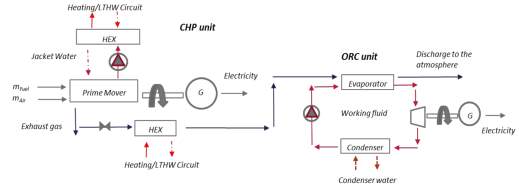
|
The dynamic model predicts the properties of the system with every crankshaft angle, by solving energy and mass balance equations. It is built within Matlab [58] used in conjunction with REFPROP [59] to calculate thermodynamic properties of the gas mixture within the system. Crankshaft angle ranges from -180-540 degrees, starting at BDC with every phase lasting 180 degrees. The phases in order is the compression stroke (-180-0 degrees, BDC-TDC), combustion with spark ignition, expansion stroke where work is generated (0-180 degrees, TDC-BDC), exhaust stroke through exhaust valves (180-360 degrees, BDC-TDC) and intake stroke of fresh air through inlet valves (360-540 degrees, TDC-BDC) starting the cycle over. To summarise with the basic equations, starting with the energy balance equation for a cylindrical open system is applied:
| dPdϑ=γ-1VQindxbdϑ-dQwdϑ-γPVdVdϑ+γ-1Vπ180ωṁintakehintake-ṁexhcyl | (1) | |
Pressure is dependent on temperature, mass and volume in accordance with the ideal gas law. As the engine runs, the piston movement changes the cylinder volume
dVdϑ, net temperature change is dependent on heat gain
Qindxbdϑand wall heat loss
dQwdϑ. Mass is determined by net flow rates from intake and exhaust valves. The instantaneous volume is further described by Eq. 2-4 with key parameters of instantaneous stroke y, maximum volume displacement
Vdisand compression ratio r. The ICE geometry is described by bore b and crankshaft length l, hence the model can simulate different engine sizes.
| Vϑ=Vdisr-1+3.14b2y0.25 | (2) | |
| yϑ=α+1-l2-α2sinϑ20.5+αcosϑ | (3) |
| dVdϑ=Vdis2sin(ϑ)(1+cosϑa2-sinϑ2)-0.5 | (4) | |
Eq. 5 describes the heat release using the Wiebe function to account for the variability that comes with the combustion process with Wiebe parameters assumed to be n=3 and
α=5[60]. Ignition timing and combustion duration is expressed in terms of crankshaft angle with subscript ign and d respectively.
| dxbdϑ=nαϑd(1-1-exp-αϑ-ϑignϑdnϑ-ϑignϑdn-1 | (5) | |
Eq. 6 gives the heat addition in terms of fuel mass and lower heating value (LHV) of methane.
| Qin=mfuelLHV | (6) |
Eq. 7 expresses heat loss through walls using the Woschni correlation [61]. It is related by the Woschni heat transfer coefficient
hg, wall area
Aw, gas temperature
Tg, wall temperature
Twand engine speed rps. These are all instantaneous values.
| dQwdϑ=hg(ϑ)Aw(ϑ)(Tgϑ-Tw)rps | (7) | |
| Awϑ=πby+π2b2 | (8) | |
The Woschni heat transfer coefficient is expressed in Eq. 9 which is dependent on pressure, piston speed, bore and temperature. The piston speed is dependent on engine speed, pressure difference and initial values of pressure, pressure and volume which is defined with subscript 0.
| hgϑ=3.26Pϑ0.8Up-0.8b-0.2Tϑ-0.55 | (9) | |
| Upϑ=2*2.28s rps+0.00324T0VdisV0P-PmP0 | (10) |
Compressible flow principles are applied to the engine where the inlet and exhaust valves are acting as nozzles. When there is compressible flow passing through a restriction it is possible for the flow to be choked, meaning fluid velocity is not able to increase further [62]. Mass flow rate can still increase by increasing the manifold pressure to increase the density of the fluid, which is also a common way to increase efficiency in ICE’s. Eq. 11 and 12 denotes the two ways of calculating mass flow for either choked or non-choked flow.
P0and
T0are upstream pressure and temperature respectively,
CDis the flow restriction coefficient due to turbulence,
Avis valve area and
γis the ratio of specific heats.
| ṁchoked=P0RT00.5CDAvγ0.52γ+1γ+12γ-1 | (11) |
| ṁnon-choked=P0RT00.5CDAvPVP01γ2γγ-1[1-PVP0γ-1γ] | (12) |
To determine if the flow is choked Eq. 13 relating upstream pressure and valve pressure needs to be calculated in terms of gamma, giving a limit. If the actual pressure relation is higher than this limit, the flow will be choked.
| PVP0=γ+12γγ-1 | (13) |
Lastly, equations for the turbocharger, which consist of a compressor and an expander, is expressed in Eq. 14-15. The turbocharger uses the exhaust gases to drive an expander and some of the power generated is used to drive a compressor to increase the inlet manifold pressure to increase efficiency. The compressor work required is calculated using inlet values of enthalpy
h0, cylinder enthalpy
h1, air mass flow and compressor efficiency. The expander work generated is calculated using exhaust and outlet values.
| Ẇcomp=ṁair(h1-h0)ηcomp | (14) | |
| Ẇexp=ṁex(hex-hout)ηexp | (15) |
3.2. Simple ORC system optimization and model
To give a better representation of the main equations used in the ORC system model, Figure 8 is repeated here with each subscript corresponding to a point in the T-s diagram.
|
|
To size the ORC system, it is required to give initial inputs for the model to optimize design point by using pinch point analysis and the constraints given by Eqs. 26-31. This will allow the optimization to determine the temperature drop and hence evaporator output. Figure 8 is not entirely representative of the actual modelling process because the heat exchanger modelling compartmentalizes the evaporator into three main sections, the preheater (States 2-3l), two phase evaporator (States 3l-3v) and superheater (States 3v-3). More detail will be given in the HEX section, but the key thing to note is that the line 5-6 will be more stepwise and have points above the respective points in the refrigerant side. The distance between these points denotes the pinch and the smaller the pinch, the larger the HEX area required. It is the optimizer that determines the optimal operating parameters such as condenser/evaporator pressures. The optimizer also determines the optimal pinch to determine the highest heat transfer achievable.
| Q̇evap=ṁref(h3-h2) | (16) | |
| Q̇evap=ṁhscp,ex(T5-T6) | (17) | |
Eqs. 16-17 are combined to calculate the optimal mass flow rate on the working fluid side. This is determined at the end of the optimization after the evaporator and condenser pressure have been set, temperature drop determined and with exhaust mass flow and constant of specific heat simulated from the CHP model.
| SHD=T3-T3vT5-PPevap-T3 | (18) |
From calculating the optimal pinch point, the superheating degree can be determined from Eq. 18. Together with condenser pressure, evaporator pressure, expansion ratio and evaporator pinch points it denotes the initial inputs to start the optimization of these parameters. There are other inputs that are set to be constant in the optimization, such as condenser pinch point, pump, expander and generator efficiency as presented in Table 6. Eqs. 19-25 calculates the work output of the expander, work requirements of the pump, net-work and condenser heat output. The equations are straightforward and additional details can be found in Ref. [12].
Table 6 Model constants and limits
| Condenser Pinch Point | Pump Efficiency | Expander Efficiency | Generator efficiency | Pressure limits |
| 10 | 0.65 | 0.7 | 0.9 | 0.95
Pcrit |
| Ẇexp=ṁref(h3-h4) | (19) | |
| ηexp,is=h3-h4h3-h4s | (20) |
| ηORC=ẆnetQ̇evap | (21) |
| Ẇexp=ṁref(h3-h4s)ηexp,isηg,el | (21) |
| Q̇con=ṁref(h4-h1) | (22) |
| Q̇con=ṁcwcp,w(T8-T7) | (23) |
| ẆORCPump=ṁref(h2-h1)ηORCPump | (24) |
| Ẇnet=Ẇexp-ẆORCPump | (25) |
| Maximise:Ẇnet
With the constraints: 0≤SHD≤1 |
(26) | |
| (27) | ||
| PevapPcon≤rexpγ | (28) | |
| Pcon |
(29) | |
| T4v≤T4 | (30) | |
| PPmin≤PP | (31) | |
For the constraints, the superheating degree (Eq. 26) is restricted being between 0-1 due to normalization as expressed in Eq. 18, which is a ratio between actual and maximum superheating [30]. Eq. 28 ensures isentropic expansion, while Eq. 29 preserves cycle conditions such as condenser pressure being lower than evaporator pressure and evaporator pressure lower than critical pressure to maintain sub-critical conditions. Eq. 30 ensures that the expansion process does not expand to the right inside the vapour-liquid dome on the T-s diagram and the temperature after expansion is higher or equal to the condenser saturation temperature. A real process always goes towards the right as shown from point 3-4. The model gives back a minimal pinch point, anything below this is not achievable as the HEX area would increase significantly. Eq. 31 ensures non-violation of this minimum pinch.
3.3. Recuperative ORC system optimization and model
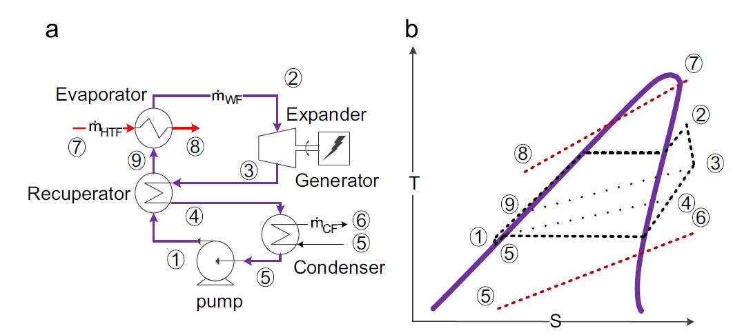
Figure 9 (a) ORC system with recuperator schematic (b) T-s diagram of system [19] |
Figure 9 shows the recuperative ORC system that will be modelled. It uses the same base equations as the simple cycle, but adds Eq. 32 to calculate the parameters at the new points. Two additional points in the recuperator T-s diagram is a point 4 further down the line and point 9 further up the line. The model assumes an effectiveness, 0.8 in this case [63]. This allows the enthalpy change to be calculated where from REFPROP the new temperature can be calculated. The enthalpy change is the same on both sides.
| ε=qqmax=h3-h4h3-h1 | (32) |
3.4. Heat exchanger sizing and part load optimisation
The heat exchanger model follows the methods used by Chatzopolou [30]. As the equations are quite involved, only the references where the methods are taken from are presented for the interested reader. The pre-heater area is calculated using Dittus-Boelter equations [64]. For the superheater/desuperheater section, a method is presented by Gnielinski [65]. These two sections are relatively easy to calculate as the WF are single phase. For the two-phase evaporator/condenser, the process is much more complicated as the liquid to vapour ratio increases the heat transfer coefficient changes. To get a more accurate number on the HEX area required for the two-phase evaporator/condenser, this section is divided into zones. The number of zones depends on the accuracy required. Additionally, five different methods are used to calculate the heat transfer coefficient of each section to calculate the total area. At the end, the mean of these method is calculated to give the final area. There are two different type of methods for tube-in-tube boiling, asymptotic method for nucleate boiling and convective boiling and one that accounts for nucleate boiling only [66]. Asymptotic method is presented by Steiner [66], Dobson [67] and Zuber [68]. As for the nucleate boiling, Cooper [68] and Gorenflo [69]. The condenser calculation follows the same approach with calculating the mean area, but using either gravity driven condensation [68], shear condensation [68] or a combination of both [77, 80].
Further to this is calculating the required pipe diameter from the known area and specifying initial velocity. From this velocity, the pipe diameter and Reynolds number can be calculated, this can calculate the length of the pipe, leading to calculating friction factor and finally the pressure drop. The pressure drop should be within the range of 1-1.5 bars. There are parameters that are required for the calculation such as density, Prandtl number, thermal conductivity and kinematic viscosity. As the parameters vary widely from pre-heater to superheater, these are all calculated from their respective sections using the temperature mean for the pre-heater and superheater. For the two-phase zone, the parameters are calculated by taking the mean of the values at vapour quality 0 and 1 as these vary relatively linearly as the fluid fully evaporates. The equations used to calculate pressure drop are [64]:
| Re= ρuDμ=uDκ | (33) | |
| L=AπD | (34) | |
| f=0.046Re-0.2 | (35) | |
| ∆Pdrop=4*f*LD*ρu22 | (36) |
For this study, the focus is on the influence of HEX’s on part load operation of ORC systems. All CHP outputs are known and it is this variation fed to the ORC system that needs to be calculated. The part load calculation for this study tries to avoid the inevitable pump efficiency and pressure variation when the mass flow of the ORC system load decreases, as can be seen in pump curves. The expander follows the same trend with its own expander curves. The main assumption for part-load operation is that the points in Figure 8-9 are constant and only working fluid mass flow changes with the CHP exhaust mass flow rate and temperature. As Calise, Capuzzo and Vanoli [71] notes it is the mass flow rate that has the most influence on the off-design, which grants leniency in terms of reduced pump and expander performance. Keeping turbine inlet temperature constant is a common assumption in calculating part load, but was found to have less influence for dry fluids than for wet fluids where it is vital for comparison sake [42]. Other general assumptions include steady-state, negligible pipe fouling, gravity terms, heat loss to environment of pump and expander. There will be a discussion on how the overall cycle changes with part load in later sections, but for the purposes of the HEX influence the cycle points are kept constant. The condenser cooling water temperatures were kept constant at 15 °C at inlet and 25 °C at outlet.
Since the cycle points are kept constant, only the outlet temperature of HEX on the exhaust side is unknown and changing. To determine this temperature and hence the actual refrigerant mass flow rate requires an iteration process as mass flow rate changes, the velocity changes and hence Reynolds number changes. Pressure drop does not need to be recalculated since velocity always decreases with mass flow rate in this case, but the heat transfer coefficient needs to be recalculated. In combination with the fixed area from the optimizer allows the iteration to proceed. The iteration steps are:
- Assume initial
T6for Eq. 17 to calculate
Q̇evap.
- From known pressure, temperature, enthalpy and
Q̇evapas they are constant, use Eq. 16 to calculate the mass flow rate.
- Calculate LMTD for each evaporator section (counter flow arrangement).
| ∆TLMTD=Th,o-Tc,i-(Th,i-Tc,o)ln(Th,o-Tc,i)(Th,i-Tc,o) | (37) |
4. Calculate new
Q̇evap. There is an inner and outer pipe area, inner area is used for the refrigerant side and outer area for the exhaust side. The outer area is calculated in much the same way as the inner area. Hydraulic diameter is used in this case for calculating the outer parameters, such as Reynolds number and Nusselt number. The equations used are:
| Q̇evap=UA∆TLMTD | (38) | ||||
| U=1ho+1hi | (39) | ||||
| Nu=0.023Re0.8Pr0.4 | (40) | ||||
| hi/o= Nui/o*kDi/o | (41) | ||||
5. Recalculate
T6. Compare to initial
T6until converged answer is reached.
With these steps, the ORC system part load curve can be found.
3.5. ORC module costing technique
There is a lack of data when it comes to costing of ORC systems, hence a cost correlation by considering each component separately before summing is required to calculate the specific investment cost. F accounts for manufacturing, while Z is component specific attribute [30].
| Cp0=F10K1+K2log10Z+K3log102Z | (42) | |
| Cp0=Fexp(K1+K2lnZ+K3ln2Z+K4ln3Z+K5ln4Z) | (43) |
Eq. 42 is a correlation that is derived by Turton et al. [43], while Eq. 43 is derived by Seider et al. [44].
| S=νwf0.0631P0.02990.5 | (44) |
Here S is the specific attribute for the pump, that accounts for design properties, such as pressure head (bar) and volume capacity (L/s). Table 7 shows the rest of the values for the constants.
Table 7 Cost coefficients for cost correlation equations [30]
| Unit | Unit attribute (Z) | F | K1 | K2 | K3 | K4 | K5 | Ref. |
| Evaporator/ condenser | Area (m2) | 1 | 9.5638 | 0.532 | -0.0002 | [43] | ||
| Preheater/ desuperheater | Area (m2) | 1 | 10.106 | -0.4429 | 0.0901 | [43] | ||
| Expander | Power (kW) | 3.5 | 2.2486 | 1.4965 | -0.1618 | [44] | ||
| Pump-Motor | Power (HP) | 1.4 | 5.83 | 0.134 | 0.0533 | 0.0286 | 0.00355 | [43] |
| Pump | S (gpm
fthead) |
2.7 | 9.2951 | -0.6019 | 0.0519 | [43] |
As the calculated cost from Eqs. 33-34 are in dollars adjusted to their specific published year, 2001 for Turton [43] and 2006 for Seider [44], there is a need to adjust for inflation using CEPCI and currency conversion into pounds. Table 8 shows the conversion factors to adjust for inflation.
Table 8 Conversion table for currency and inflation
| Value | Reference | |
| Currency conversion 2001 | £1=$1.84 | [30] |
| Currency conversion 2006 | £1=$1.439 | |
| CEPCI-2001 | 397 | |
| CEPCI-2006 | 500 | |
| CEPCI-2017 | 562 | [72] |
Chapter 4. Results and discussion
4.1. CHP model validation
Three engines with different capacities were modelled and validated against real engine data from Ener-G accounting for the capacity of CHP-1520 [73], CHP-502 [74] and CHP-310 [75]. The data sheet only gives information for 100%, 75% and 50% load, which means the 90%, 80% and 60% values had to be calculated assuming constant AFR. The model gave results that made this assumption a reasonable choice to find the fuel heating value, fuel and exhaust flow rate. Since these values are outside the data sheet, the comparative real value against model value is an estimation. For example, the actual heat output for 90% if found by multiplying with 90% of the 100% value. The data sheet themselves gives a percentage tolerance to the value given and can vary up to 10% depending on what data investigated. Efficiency have 5% tolerance, electric power 3% and heat output 10%. The results presented in the next few pages are separated by engine capacity, showing efficiency, power, exhaust mass flow and temperature and exhaust and cooling circuit output comparisons. Most of the comparisons were within this tolerance except for exhaust and cooling circuit outputs of the CHP-502 and CHP-310. Despite this when summed up they do still come within the total heat output tolerance. These could in some degree be influenced by the input variables, but were negligible in most cases. The different capacity engines see the same trends. Figure 10-12 show the efficiency variation of the CHP with part load for CHP-1520, CHP-502 and CHP-310 respectively.
|
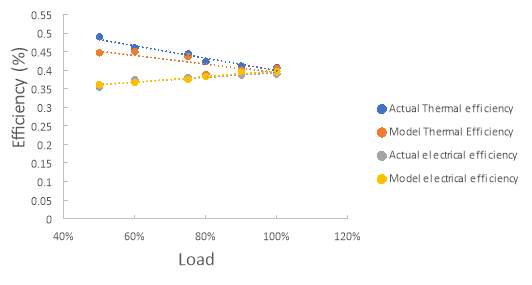
Figure 11 Part Load efficiency comparison CHP- 502 kW
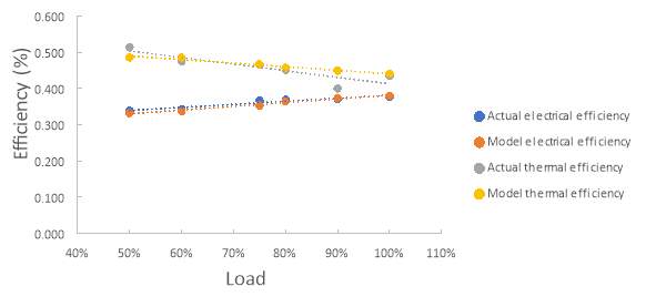
Figure 12 Part load efficiency comparison CHP-310 kW
The CHP engine is optimized for electrical power. As load decreases, the electrical efficiency will decrease. This occurs because the engine is being less efficient in utilizing the fuel available, wasting potential work and subsequently more heat is released to the environment. For this reason, as heat increases, the thermal efficiency increases with decreased load. Ignition timings is a very important variable as too early ignition can make the upward stroke of the piston work against the expanding gases from combustion leading to decreased efficiency. Too late ignition can result in reduced ignition duration and lead to incomplete combustion as valve opens and overlaps. The key to ignition timing is the mixing of fuel and air. To get good combustion, a sufficient mixing is required, which is why turbulence in the cylinder is designed for. This mixing requires time and requires a balance of the duration of combustion (ignition timing not too late) and proper mixing (not too early). As a rule of thumb, the optimal ignition timing is around -4 degrees bTDC. Later ignition angle allows better blended fuel mix, which means the temperature will generally be higher as more of the fuel is utilized and efficiency increases. It can however lead to higher NOX emissions as NOX is dependent on increased temperatures. Other variables that can influence these results, but not explored are inlet and exhaust valve events. There are various advantages and disadvantages of proper timings. Valve overlap can lead to blowdown from the inlet to exhaust as inlet manifold has higher pressure, this can lead to a fuel rich mixture and increased residuals, but does reduce pump work [76]. Additionally, with blowdown the exhaust gas would be colder from the fresh air from inlet valve. Earlier exhaust valve timing allows the piston to help push combustion air out, which decreases exhaust temperature as combustion gases is in the cylinder for a decreased duration. Later exhaust valves off, reduces electrical output because of bypassing from valve overlap, also have higher exhaust mass flow.
When comparing the actual efficiencies against the model efficiencies, the trends are going the same direction with decreased load as shown in Figure 10-12. However, as CHP-1520 has a more exponential trend, while CHP-502 and CHP-310 have linear trends. The estimation of the part load values does come more into light as capacity decreases and it is possible the model is not accurate below a certain capacity.
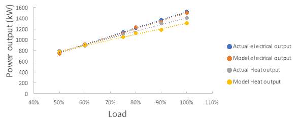
Figure 13 Part load power comparison CHP-1520 kW
|
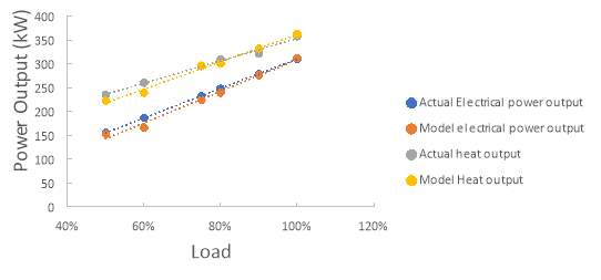
Figure 15 Part load power comparison CHP-310 kW
Figure 13-15 show the part load power output of the CHP for the different CHP capacities. The part load power comparison is all similar and as expected do vary linearly as presented in Figure 13-15. Although the heat output seems to vary in the same manner as the electrical output, meaning one would expect electrical efficiency to have the same trend. However, the fuel input also decreases. The ratio of heat to electrical output with heating value increases leading to the thermal efficiency to be higher than electrical efficiency as the ICE becomes less efficient in fully utilising the fuel.
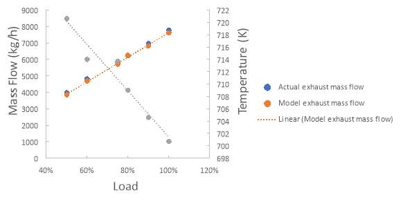
Figure 16 Exhaust mass flow part load comparison CHP-1520 kW
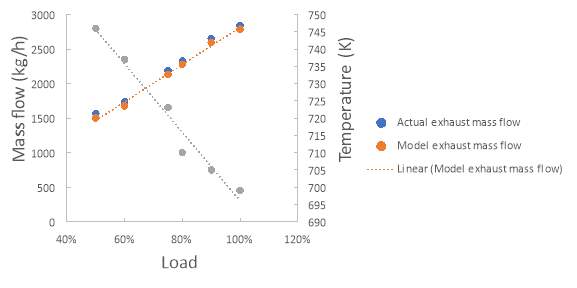
Figure 17 Exhaust flow part load comparison CHP-502 kW
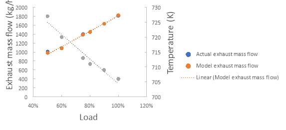
Figure 18 Exhaust flow part load comparison CHP-310 kW
Figure 16-18 illustrate the exhaust flow rate and temperature variation with part load of the CHP’s. Key observation for the exhaust flow is the increase of temperature as load decreases, presented in Figure 16-18. This is again because of reduced utilisation of the fuel to do work. Exhaust flow rate decreases with part load as less power output require less fuel and hence less air, which leads to a net decrease of exhaust mass flow rate.
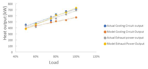
Figure 19 Exhaust and cooling circuit output comparison CHP-1520 kW
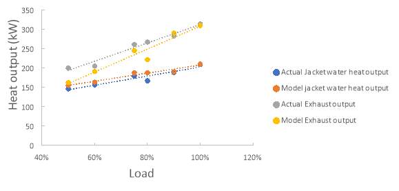
Figure 20 Exhaust and cooling circuit output comparison CHP-502 kW |
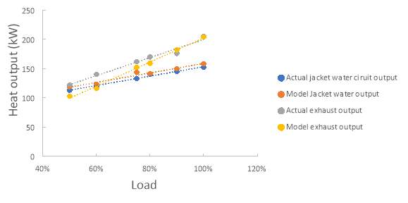
Figure 21 Exhaust and cooling circuit output comparison CHP-310 kW |
Figure 19-21 illustrate the exhaust and cooling circuit output comparison of the CHP’s, following the same trend as the heat output, but the interaction of valve and ignition timings is quite involved. The theory around it has already been mentioned, but is mostly determined by how long the combustion gases stays in the cylinder. The longer the combustion gases stays in the cylinder, the more losses to the walls and cooling water circuit. As losses increases, the exhaust gas temperature will decrease. The results do show good correlation between the actual engine and model data and hence have been validated. Three different capacities were tested to investigate the applicability of the model as simulating small and large engines can lead to difficulties. In this case, the model performed well, though the heat output from the cooling circuit and exhaust gas could indicate that it is at its limits. Future testing on lower capacities is required to test for model robustness.
4.2. Analysis of optimized ORC system results
For both the recuperator and simple cycles, the ORC system values are optimized according to several CHP loads. The optimization determines the design point otherwise known as the 100% load of the ORC system. This can be optimized against a range of CHP loads, ranging from 50-100%. This means if the 100% CHP load values are chosen, it will correspond to the 100% load of ORC system. This can continue with 90% CHP load values that will ultimately correspond to 100% load of the ORC system and so on. Various of these tests are done to get the best range of options for future economic optimization. The reason why the ORC system is not just optimized against 100% CHP load is because on majority of cases the CHP will run at 75-90% load and only in rare cases will it run at 100% load, even at peaks. Running a system at design point is always desirable for optimal efficiency and as mentioned in the CHP prime mover section, ICE operates at relatively constant efficiency even at part load. What load to optimize against ultimately relies on the demand required and if the buffer to full CHP load is adequate, a larger sized ORC might not be required. This might also depend if there is a requirement for the system to grow. Table 9-14 shows the different operating parameters, output and efficiency of different fluids for an optimized cycle for simple and recuperated ORC cycle optimized against CHP-1520kW, CHP-502kW and CHP-310kW respectively.
Of the initial 5 working fluids tested, R1234ZE and P-Xylene gave the lowest power output and efficiency as shown in Table 10-11 and same trends was found for the other engine sizes. Hence, Toluene, R1233ZD and Benzene were the three chosen for further analysis. The values in Table 6 show the power output optimized against the CHP load and other key parameters of note. To clarify for the power output column in Table 8-13, the percentage refers to the CHP load that the ORC is optimized against. The values given are the 100% ORC system load net-work for that CHP load respectively. The results are presented capacity wise. The table also shows the pressures that occurs the most for that fluid. It is important to note that for the simple ORC system, Toluene is the only fluid that show significant difference in operation conditions when optimized against different CHP loads, especially for evaporator pressure. The evaporator pressure received in some simulated conditions an optimal evaporator pressure of 2950kPa. It is uncertain why these cases occur, but it only gives a slight increase in power output and efficiency. There is little difference of results for different CHP capacities, the only difference being smaller ORC system as less heat is available. Efficiency is the same for each fluid and cycle.
Table 9 Optimised ORC system values for the simple ORC cycle (For CHP-1520 kW)
| Working fluid | Power output (kW) (75%/80%/90%/100%) | Pump Work (kW) | Condenser pressure (kPa) | Evaporator pressure (kPa) | Gamma | Efficiency |
| Toluene | 71.51/77.13/86.1/91.5 | 3.7 | 50 | 977 | 1.1 | 0.121 |
| R1233ZD | 74.97/80.9/86.93/96 | 12.5 | 159 | 3394 | 1.13 | 0.126 |
| Benzene | 90.5/97.6/104.9/115.8 | 7.4 | 50 | 2178 | 1.39 | 0.152 |
Table 10 Optimised ORC system values for recuperated ORC cycle (For CHP-1520 kW)
| Working fluid | Power output (kW) (75%/80%/90%/100%) | Pump Work (kW) | Condenser pressure (kPa) | Evaporator pressure (kPa) | Gamma | Efficiency |
| Toluene | 73.8/79.4/85.3/94.2 | 3.8 | 50 | 977 | 1.1 | 0.142 |
| R1233ZD | 92.6/99.7/107.2/118.3 | 15.6 | 175 | 3394 | 1.12 | 0.174 |
| Benzene | 98.6/106.2/114.2/126.2 | 8 | 50 | 2178 | 1.39 | 0.176 |
The power output variation between fluids and CHP loads is influenced by the exhaust mass flow more than the temperature. As exhaust mass flow of the CHP decreases with load, the optimal mass flow rate of the refrigerant also decreases to accommodate this. The WF power output variation for the simple ORC cycle is because of the gamma value, which is the ratio of specific heats for constant pressure and volume. The expander work depends on the fluid pressure ratio and it respective evaporator temperature. A higher gamma value allows a higher operating cycle pressure ratio. For the simple ORC system, the gamma of Toluene and R1233ZD are similar and get similar output. Gamma for Benzene however is higher giving a power output advantage ranging from 8-20kW. The Gamma for the fluids are shown in Table 8-13 for their operating points.
The recuperator cycle is different, relying less on the gamma value and more on the increase of optimal mass flow rate of the refrigerant. As a recuperator is incorporated, there is an increase in mass flow rate to take advantage of extra heat from the exhaust of the CHP, but also leads to an increase in net work. The biggest difference is for R1233ZD as it is the only fluid with large degree of superheating. This allowed for better utilization of the waste heat as there was more heat available to heat the liquid phase as seen in the T-s diagram of Figure 9 compared to Toluene and Benzene. R1233ZD saw the highest increase in mass flow rate in that regard and getting equal to Benzene in terms of output and efficiency. R1233ZD is the only fluid with significant superheating as it has the lowest latent heat of the three, meaning it has the narrowest dome. In short, it means it evaporates quickly allowing superheating to occur. R1233ZD’s mass flow rate is also significantly more than the other two fluids. Even so, it is also the densest, requiring larger pump work and is the reason for R1233ZD not having the highest net-output overall. The pump work for 100% is shown in Table 8-11 for comparison. As mass flow rate decreases with the decreased CHP load it is optimized against, the pump work decreases with the same trend as illustrated in Figure 22.
Table 11 Optimised ORC system values for the simple ORC cycle (CHP-502 kW)
| Working fluid | Power output (kW) (75%/80%/90%/100%) | Pump Work (kW) | Condenser pressure (kPa) | Evaporator pressure (kPa) | Gamma | Efficiency |
| Toluene | 26.8/28.1/32.5/35 | 1.4 | 50 | 977 | 1.1 | 0.121 |
| R1233ZD | 27.3/29.5/34.1/36.7 | 4.8 | 159 | 3394 | 1.13 | 0.126 |
| Benzene | 32.9/35.6/41.2/44.3 | 2.8 | 50 | 2178 | 1.39 | 0.152 |
| P-Xylene | 22/23.8/27.5/29.6 | 1.3 | 50 | 936 | 1.08 | 0.11 |
| R1234ZE | 18.1/19.6/22.7/24.41 | 4.6 | 573 | 3453 | 1.11 | 0.084 |
Table 12 Optimised ORC system values for recuperated ORC cycle (CHP-502 kW)
| Working fluid | Power output (kW) (75%/80%/90%/100%) | Pump Work (kW) | Condenser pressure (kPa) | Evaporator pressure (kPa) | Gamma | Efficiency |
| Toluene | 26.8/29.1/33.6/36.3 | 1.5 | 50 | 977 | 1.1 | 0.142 |
| R1233ZD | 33.7/36.5/42.2/45.5 | 5.8 | 174 | 3394 | 1.12 | 0.175 |
| Benzene | 35.9/38.9/44.9/48.4 | 3.1 | 50 | 2178 | 1.39 | 0.176 |
| P-Xylene | 22.8/24.8/28.7/31 | 1.36 | 50 | 936 | 1.08 | 0.138 |
| R1234ZE | 25.1/27.1/31.3/33.8 | 7 | 634 | 3453 | 1.11 | 0.124 |
For the condenser pressure, it is in some degree connected to the critical temperature of the fluid, but in the modelling of the ORC system in case, is limited to 50kPa. As critical temperature increases, a lower condenser pressure can be achieved [77]. The critical temperature of Toluene and Benzene are similar and hence have the same condenser pressure. R1233ZD have a lower critical temperature and has a higher condenser pressure. In most cases, an atmospheric condenser pressure is desirable to prevent leakage. For Toluene and Benzene with the lower condenser pressure, the latent heat is higher the lower the pressure, leading more heat to be rejected to the environment, which is undesirable. A fluid with a high latent heat at lower pressure will lead to lower efficiency [77]. The higher condenser pressure of R1233ZD can give leakage issues, but as it is one of the refrigerants with no ODP and low GWP the environmental impact of potential leakage is lower than other fluids. Evaporator pressure is a result of critical pressure and pinch point. R1233ZD operates close to its critical pressure to get an optimal pinch point that is line with Toluene and Benzene. This is because refrigerants generally have a T-s diagram dome that are smaller than hydrocarbons as their intended operation is for refrigeration and not power generation. It is from this perspective that makes the different operating pressures of Toluene make little sense, as the low pressure of Toluene should have a higher optimal pinch point. Looking at the HEX sizes presented in the next section however does explain how this is possible as Toluene gets the highest HEX area requirements.
Table 13 Optimised ORC system values for the simple ORC cycle (CHP-310 kW)
| Working fluid | Power output (kW) (75%/80%/90%/100%) | Condenser pressure (kPa) | Evaporator pressure (kPa) | Gamma | Efficiency |
| Toluene | 16.6/17.1/19.6/22 | 50 | 977 | 1.1 | 0.121 |
| R1233ZD | 17.1/17.9/20.6/23.1 | 159 | 3394 | 1.13 | 0.126 |
| Benzene | 20.7/21.6/24.8/27.9 | 50 | 2178 | 1.39 | 0.152 |
Table 14 Optimised ORC system values for recuperated ORC cycle (CHP-310 kW)
| Working fluid | Power output (kW) (75%/80%/90%/100%) | Condenser pressure (kPa) | Evaporator pressure (kPa) | Gamma | Efficiency |
| Toluene | 16.7/17.9/20.8/22.7 | 50 | 977 | 1.1 | 0.142 |
| R1233ZD | 21/22.1/25.3/28.5 | 174 | 3394 | 1.12 | 0.174 |
| Benzene | 22.5/23.6/27/30.4 | 50 | 2178 | 1.39 | 0.176 |
Efficiency is the most complex in terms of parameters affecting it. There was found a weak correlation between critical temperature and efficiency by Liu et al [23], having found that a lower critical pressure leads to a lower efficiency, but also an increase in efficiency with heat source temperature. The boiling temperature also influences efficiency for fluids operating at the same pressure with the higher boiling temperature fluid having higher efficiency [78]. As for the interpretation of the results given in Table 8-13, the efficiency is dependent on how effective the fluid is to extract heat from the exhaust to what it can generate in power. This is dependent on the thermal conductivity and specific heat, where Toluene and Benzene are similar and R1233ZD has a smaller value. The recuperator gives better efficiency as the heat is utilized more efficiently and less heat is required in the pre-heater section leading to better efficiency in correlation with Eq. 21. Although R1233ZD is the only fluid with significant superheating, all dry fluids do in some degree have heat to spare represented by the area marked by the points 3-4-4v in Figure 8, which is why R1233ZD gained the most out of installing a recuperator as the fluid had largest degree of useful heat at expander outlet. In a sense, there is a heat transfer efficiency that determines how effective the fluid can extract the heat from the exhaust gas. A fluid that require more mass flow rate to get the same amount of heat is deemed to be less effective. How much fluid required depends on the thermal conductivity of the fluid and specific heat. The specific heat determines how much heat the fluid can contain, if it is low, more mass is required to hold the same amount as for a reference fluid. As for thermal conductivity, it determines how quickly the heat can transfer through the fluid. In both cases, 1233ZD has a lower value at operational points. It was found that these values were accurate within 1% when compared to industry when it came to sizing the ORC system as noted by Chatzopolou [11].
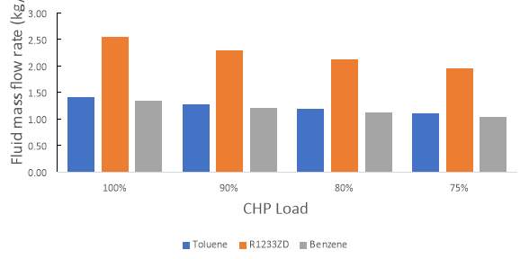
Figure 22 Optimised flow rates comparison with CHP load (CHP-1520 kW, ORC with recuperator) |
4.3. Heat exchanger sizing results and analysis
Figure 23-27 illustrates the different HEX areas of evaporator, condenser and recuperator, for simple and recuperated CHP-1520. The HEX size for each fluid depends on several criteria. The first criterion is unrelated to the fluid, the LMTD. A higher LMTD denotes a higher thermodynamic drive or more simply a higher temperature difference making it more efficient in transferring heat and therefore will require less HEX area. The HEX area values that is shown from Figures 23-27 do not tell the whole story as they do not tell the proportion of the sizes of the preheater, evaporator and superheater. Simply, the preheater always has the largest proportion, followed by evaporator and superheater respectively. Table 15-16 shows the LMTD for the various sections for the different fluids for simple ORC and ORC with recuperator respectively, which correlate well with low LMTD having a larger HEX area. The correlation between area and LMTD has a linear trend in that regard. The HEX area decreases linearly depending on what load condition the ORC system is optimized against as seen in Figure 23. The only exception is for 75% CHP load for Toluene where it increases. The optimizer identified a different optimal operating point, having a higher evaporator pressure, which gives a smaller pinch point. To achieve these smaller pinch points, the HEX area needs to be larger and in an ideal case, the area goes to infinity when the pinch point is zero, hence can never be achieved. Although the optimizer gives an optimal pinch point, it is only a recommended value and a bottom limit, both for economic and size reasons. There is no ceiling, but will be less efficient the higher the pinch point.
Table 15 LMTD for simple ORC system
| Working Fluid | LMTD preheater | LMTD evaporator | LMTD superheater |
| Toluene | 20 | 107.6 | 204 |
| R1233ZD | 78 | 124.5 | 161 |
| Benzene | 43 | 117.5 | 200 |
The preheater in the case of the simple ORC system accounts for 86% of the total evaporator HEX area. As the evaporator increases, the latent heat decreases and is why the preheater area tend to be significant. For every case of Toluene, the superheating degree is zero and therefore has no superheater section. R1233ZD is the only fluid that has a noticeable superheater area because of its low latent heat of vaporization compared to Toluene and Benzene.

Figure 23 Evaporator area optimised against CHP load comparison (CHP-1520 kW) |
Toluene exhibits a considerably larger HEX area than the other fluids. This is all in the preheater, having the lowest LMTD for that section. The correlation between LMTD and size is relatively linear, the same area for Benzene is about half the number of Toluene and R1233ZD is about one quarter the value.
For the ORC with recuperator, there is a marked decrease in total evaporator area due to the incorporation of a recuperator. For Toluene, a small recuperator of 3.5 m2 effectively removes about 70% preheater area when comparing Figure 23 and 24. The benefits of a recuperator for dry fluids is paid off immediately, though has varying benefits depending on the fluid. There is less size benefit for R1233ZD and Benzene, although it is still significant, the main benefit for these two fluids lie in the efficiency gains, which will benefit economically for capital cost and operational cost. The operational cost is not considered for this thesis.
Table 16 LMTD for recuperated ORC system
| Working Fluid | LMTD preheater | LMTD evaporator | LMTD superheater |
| Toluene | 17.9 | 107.9 | 218.5 |
| R1233ZD | 20.5 | 75.5 | 133 |
| Benzene | 19 | 106.5 | 200 |
The second criterion has already been discussed, the pinch point, which is specific to the fluid. This is because the fluid determines the evaporator pressure, therefore how close it is operating against the exhaust gas temperature. The T-s diagram domes of Figures 8-9 are not entirely representative of where the pressure lines would occur. The domes of Toluene and Benzene are wider and taller than R1233ZD, but the pressure line for R1233ZD’s operating state can still be lower than the one for Toluene and Benzene. This trend is a culmination of many characteristics such as density, molecular weight, critical temperature and many others. Generally, a higher pressure does not necessarily mean higher efficiency, but will allow less heat requirements due to latent heat of vaporization reduces with increased pressure and higher power output. One of the benefits of ORC’s is that it can operate at lower pressures than steam cycles, meaning cheaper, more compact systems because less material requirements as it doesn’t need to handle as high pressure.
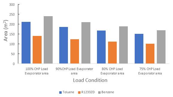
Figure 24 Evaporator area optimised against CHP load comparison (CHP-1520 kW, ORC with recuperator) |
For the recuperator, there is a marked decrease in total evaporator area due to the incorporation of a recuperator. For Toluene, a small recuperator of 3.5 m2 effectively removes about 60% when comparing Figures 23 and 24. The benefits of a recuperator for dry fluids is paid off immediately, though has varying benefits depending on the fluid. There is less size benefit for R1233ZD and Benzene, although it is still significant, the main benefit for these two fluids lie in the efficiency gains, which will benefit economically for capital cost and operational cost. The operational cost is not considered for this thesis.
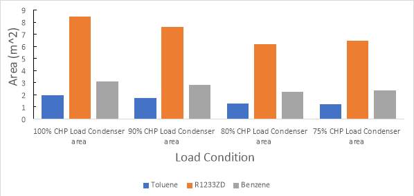
Figure 25 Condenser area optimised against CHP load comparison (CHP-1520 kW)
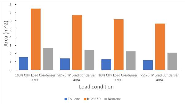
Figure 26 Condenser area optimised against CHP load comparison (CHP-1520 kW, ORC with recuperator)
The third criterion is the thermal conductivity of the fluid. It is similar for Toluene and Benzene, but for R1233ZD it is lower. It gives a lower Nusselt number and hence a lower overall heat transfer coefficient. Reducing the overall heat transfer coefficient and keeping the evaporator output and LMTD constant in Eq. 38 leads to a higher area requirement. It is not well represented in the results here as the optimizer, rather than increasing HEX area, increases the mass flow rate in accordance with Eq. 16. If the mass flow rate and operating pressure was to be kept the same for all fluids, the area variation would be clearer. This is highly unlikely as they operate optimally at different conditions and hence there will be no further discussion of this topic.
The fourth criterion is the Prandtl number, which is the ratio between momentum diffusivity and thermal diffusivity. It is effectively an indicator of whether heat transfer by conduction or convection is dominant for a fluid state. For all three fluids, having Prandtl number less than 1, conduction is the dominant heat transfer method for the fluid, but it is quite close to 1 and therefore both heat transfer methods do, to some degree, influence the process. The Prandtl number influences the Nusselt number, which again influences the overall heat transfer coefficient. As Nusselt number is related to convection more than conduction, the low Prandtl number only lead to lower convective heat transfer coefficient. A fluid being conduction dominant benefit more from a large area rather than mass flow rate that convection dominant fluids can exhibit.
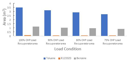
|
Technically, Prandtl number is dependent on thermal conductivity and viscosity. Viscosity is a key factor for Reynolds number with a lower viscosity giving a higher Reynolds number, which increases Nusselt number. It also decreases pressure drop which is vital to determine the efficiency of the system. A lower pressure drop requires lower pump work, making it more efficient, hence a lower viscosity is preferred for systems of this purpose. Oil is very viscous and is more effective in convective heat transfer. It is usually the fluid of choice in terms of cooling circuits because of this and having a low evaporating pressure to allow high degree of cooling where water is not readily available or inappropriate, as large amounts is generally required and a small system is not able to accommodate.
There has been little discussion on the differences between the different ICE engines of varying capacity. This is because the trend is the same, so a general explanation will suffice. The main thing is a linear decrease of HEX size with engine capacity as less heat is available. The condenser requires less area compared to the evaporator as water is a very effective cooling fluid. Water can be convection dominant so having more mass flow over the pipes is more effective. The mass flow rate of the gas and water sides of the pipes were both optimized with a starting point of 30 kg/s, which is significantly higher than the WF side. The optimizer chose the lowest condenser pressure to achieve highest pressure ratio, but it does have its downsides as lower pressure has higher latent heat, leading to more heat being rejected. As for why R1233ZD requires larger condensers compared to Toluene and Benzene, it is because the mass flow rate of R1233ZD is higher and hence a larger area is required to cool it.
4.4. Part load performance of the simple and recuperated ORC system
4.4.1. The influence of the HEX on the ORC system
The results in this section illustrates how the HEX influences the power output and efficiency with decreased CHP load. As it is the CHP that is sourcing the heat for the ORC system it makes more sense to show the CHP part load instead of the ORC part load. Additionally, as the ORC system is driven by the CHP, a decreased load will not automatically mean that the efficiency will drop. In fact, as can be observed in Figure 28-29, the efficiency increases with decreased CHP load. The trend translates to the overall net-work drop associated with a decrease in mass flow rate, was proportionally lower than the heat extracted at the evaporator. This is a consequence of the properties change of the exhaust gas (temperature and flow rate) when the ICE CHP going part load. Although the mass flow rate decreases, there is a subsequent increase of temperature as fuel utilization worsens. This temperature increase is more substantial than the mass flow rate in this case, leading to the trend that can be seen in the results. The iteration process was used to find a more accurate temperature of the outlet for the part load condition and in all cases led to substantial increase compared to full load, with as much as 80 degrees in some cases. This increase overall led to a smaller temperature difference as described by Eq. 17, giving a smaller evaporator output, leading to an increased efficiency in accordance with Eq.21. With the CHP giving outputs following the trends explained, the HEX influence of the system increases the efficiency in all cases presented in this section.
It is important to comment that there are many variables that needs to be considered when choosing the best option, not just power output and efficiency. The best way to do this is a thermo-economic analysis, but to do this require more data on actual ORC systems available to validate against. The optimized ORC system outputs vary greatly and it is not certain that these specific sizes exist in the ORC market. At worst case, companies can design one to match the specification of the optimizer, although it is unlikely and will incur extra cost in that case. Finding the closest match will inevitably change the system, giving rise to a bigger uncertainty. The influence of condenser is not discussed here because the water side of the condenser assumes constant inlet and outlet turning the fluid back to saturated liquid. The main interest is in the evaporator and interaction with exhaust gas, hence the condenser side is not part of the analysis.
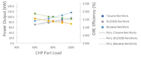
Figure 28 Simple ORC system comparing part load performance of different WF optimised against 100% CHP-1520kW load |
There is a different trend between the simple and recuperated system as can be observed in Figure 28-29. Although the form is slightly similar, the trends for the recuperated ORC system is more prominent for the power output. It is not certain why the simple ORC system gives relatively simpler trends than the recuperated system, though it is possible that the ORC with recuperator is more sensitive to an initial change in load. There is a big drop in power output for the recuperated system compared to the simple system then proceed to show the same trend afterwards. It is possible that the higher initial mass flow of the recuperator can only be upheld at full load and hence the initial drop is significant for the recuperated system only.
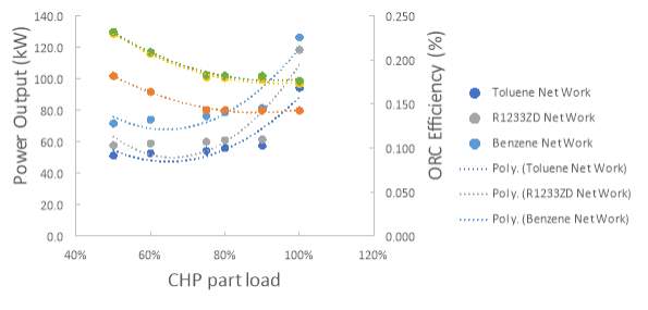
Figure 29 Recuperated ORC system comparing part load performance of different WF optimised against 100% CHP-1520kW load |
There is relatively minor change in power output when running at part load after the initial drop to 90% load. Afterwards, there is only a minor change, which seem to mean that it gives a relatively constant output. It is uncertain whether this reflects real application or if the exhaust gas mass flow rate and temperature change is indeed resulting in this trend. Without industrial data to validate against it is an unknown, which reinforces the need for additional data.
4.4.2. Comparison of overall heat transfer coefficient
Figure 30-31 illustrates the overall heat transfer coefficient variation at part load for simple and recuperated ORC system respectively. The simple and recuperated system show opposite trends both in fluid variation and direction. For R1233ZD, the overall heat transfer coefficient is relatively constant for the simple system, while it has a larger variation for the recuperated system and opposite for Toluene and Benzene. It is important to note that the overall heat transfer coefficient presented is one calculated using the LMTD and area of the entire system combined as the variation would be too high otherwise. As the operating points are kept constants for the ORC system, only velocity is changing at the ORC side, while temperature and velocity changes at the exhaust gas side. The WF mass flow rate change for the simple system is less than the recuperated system. This helps explain the difference in trend for Figures 28-29. For the simple system, the outlet temperature of the exhaust gas sees small increase, which makes sense as the extracted heat is related to the WF mass flow rate that also sees small decrease. This gives the relatively linear trend for the simple system. This gives a small change in Reynolds number for both the exhaust and WF side, giving the trend presented here. For the exhaust side, the temperature increase is small, giving a small change in thermal conductivity and viscosity. The change in overall heat transfer coefficient will hence be small, as some parameters changes, cancelling each other to some degree.
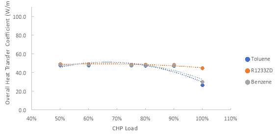
Figure 30 Overall heat transfer coefficient of the evaporator for simple ORC system |
For the recuperated system, the refrigerant mass flow rate sees a larger decrease, while the outlet temperature of the exhaust gas sees significant increase. This gives a substantial Reynolds number decrease for the WF side, giving a general decrease in overall heat transfer coefficient. The temperature increase changes the thermal conductivity and viscosity to a higher degree than the simple system, shifting the trend direction. This trend as shown in Figure 31, follows the trend in Figure 29 closely. R1233ZD is more prominent for the recuperated system as it has the most available heat to be recovered.
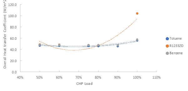
Figure 31 Overall heat transfer coefficient of the evaporator for recuperated ORC system |
4.4.3. Influence of other ORC components
To make the results presented viable for thermo-economic analysis and as a decision-making tool requires a validation process. There is a wide range of different ORC systems out in the market each with their own specifications and demands. Figure 32 shows some of the efficiencies encountered in industry against heat source temperature and as can be observed there is a wide selection of different ORC systems that is used in the TSO model by Cedillos [79]. The key indicator to take from Figure 32 is that it corresponds well with the efficiency received for the results represented for Benzene at 400 °C. It does however vary with fluid and Figure 32 does not show what fluid the ORC units are using. The different units will have a range of different types of pump, evaporator, expander, condenser and working fluids, which will inevitably change system characteristics and interactions. For example, different types of pumps include reciprocating, scroll, screw and centrifugal pumps. There is a slight issue with selecting an ORC system that is not designed to couple with a specific CHP. There is a wide range of ORC units in the market that will behave differently as their size and components differ. It becomes important to either get industrial data for validation or model every type of HEX, pump and expander to get the full picture. This thesis has studied the influence of tube in tube HEX’s from first principles and is applicable to ORC systems in the market that uses these HEX types. Additionally, it is also applicable with pumps that follow the flat characteristic curve.
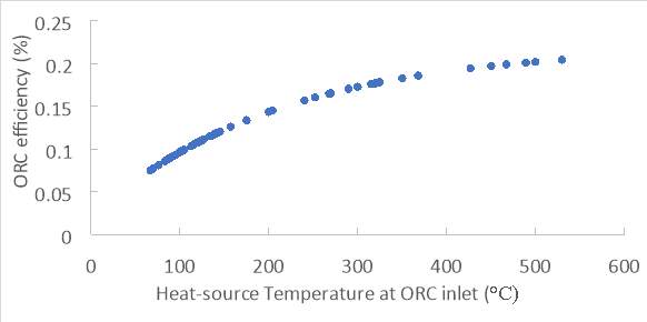
Figure 32 ORC efficiency against heat source temperature collected from industrial data [80]
Even when the focus of this thesis is seeing the influence of HEX’s on the ORC system, there is a need to discuss the influence of the pump and expander as the efficiency changes with a change of mass flow rate, which occurs at part load. This can be observed in Figure 33 on how the head or pressure increase, changes with a given flow rate. As the flow rate increases, the pressure increase that the pump can handle decreases as it has more fluid to increase the pressure of. Depending whether the pump has a steep or flat characteristic curve, it will be able to accommodate a change in flow rate better, giving the same pressure increase when the flow rate changes. As a rule of thumb the flow rate can usually change about 25% and still give the same pressure change [81]. For the part load results presented, the mass flow rate changes more than this rule of thumb, but it can be assumed that the pump follows a flat characteristic curve, giving a relatively small head change allowing for a more lenient flow change to give the same head. A relatively small head change gives small changes to fluid properties and will not affect the results significantly. As the flow rate decreases with decreased CHP load, it would mean that there will be more available head, or a pressure increase, if the speed of the pump is kept constant. Nonetheless, the outlet temperature and pump work is underestimated with these assumptions. A decrease in flow rate can also result in cavitation, which is a phenomenon that occurs when the pressure drops to a point where the fluid can naturally vaporize. The low pressure is required for the correct suction of fluid. These fluid bubbles can pop sending a concentrated stream of high velocity fluid that can damage the pump material. No definite solution has been found for this problem and will in the long run deteriorate pump performance.
A study done by Feng et al [82] investigated the operational characteristics when there is a change in mass flow rate and heat source temperature for all ORC components. Comparing the results between this thesis and the study by Feng et al [82] show very similar results in terms of how the mass flow rate and temperature changes. However, there are some different assumptions. For example, the pump can change speed and be able to adapt better to changing conditions. The key point to note from the study is how the performance of all components are enhanced by increased heat source temperature and hence it is possible some of the problems presented by the pump characteristic curve is overcome to some degree. A decrease in mass flow rate gave a lower efficiency, but is slightly rectified by the increase in heat source. These events are observed to happen in this thesis, but as the operational points are kept constant, the increased heat source might have no say after all. It can be concluded that keeping constant operational points is detrimental in illustrating what is actually happening in the process.
For these reasons, there are certain inaccuracies that comes with keeping the operational points of Figures 8-9 constant as the entire system can change because of efficiency changing for all the components. The next step following this thesis is to study the impact of pump/expander to get the full picture. There will be a general discussion on how the system would change if it was incorporated as studies on component efficiencies with part load have been investigated for standalone ORC systems [80, 81]. As efficiency decreases, more work is required to pump the fluid in accordance with Eq.24, but it also results in a higher temperature and hence less heat is needed for the preheater. As the mass flow rate decreases, pump work drops, but as efficiency decreases with pump part load, there is a slight balance between the decrease of efficiency and mass flow rate. The effect of these two cancels each other out to some degree.
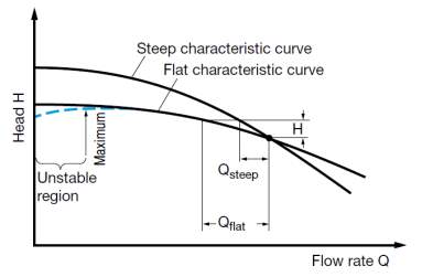
|
The expander follows in slightly the same way as the pump, but having different influencing parameters. The off-design of a turbine is complicated and can fill several papers on its own and hence the detailed process will not be discussed, only the general consequences. The key parameters are presented in Figure 34, being influenced by turbine inlet temperature, mass flow rate, turbine speed, inlet and outlet pressure. For the case of this thesis, the pressure ratio, speed and turbine inlet temperature is assumed to remain the same. This is where assuming constant turbine inlet temperature simplifies things, in the sense that only one variable changes. On the x-axis, the only thing changing in the formula is the mass flow rate and it decreases. The outer rings are efficiencies that decreases the further out you get from the middle ring. As efficiency decreases, the turbine delivers less work in accordance with Eq.21 and leads to increased temperature at the turbine outlet, which does, however, lead to more available heat for recovery in the recuperator. The outlet temperature of the expander from the model is underestimated and turbine work is overestimated for part load operation. For the expander, the effect of decreased mass flow rate and efficiency compounds leading to worse overall performance.
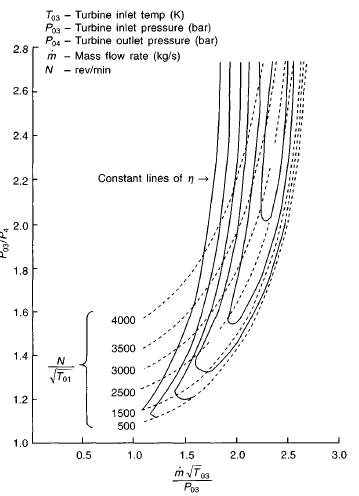
|
The ORC system optimized against 100% CHP load, have had its part load characteristics represented here. The part load curves for 75-90%% show the same trend so is not presented. The ICE CHP is assumed to be able to operate at maximum 50% capacity, hence when the part load is calculated for 75-90% only a few points remain and hence can only give part of a picture. It will depend on what the goal is for commercial application. An economic optimization will be able to determine the best configuration with the findings of this thesis and future endeavours in modelling the pump and expander. The findings in this thesis is not adequate for a full decision-making tool, but is a good start either by further modelling or collection of industrial data.
4.5. Economic analysis
Figures 35-36 show the SIC of the recuperated and simple ORC system. As the net output increases the cost decreases because of the benefit of economies of scale. Of the three fluids, Benzene is the cheapest for both systems at 2260 £/kW at 115.8 kW for the simple system and 2200 £/kW at 126.2 kW for the recuperated system. The most expensive is Toluene 5050 £/kW at 16.6 kW for the simple system and 4800 £/kW at 16.7 kW for the recuperated system, while R1233ZD lies in the middle of the SIC range. It is important to note that this is based purely on fluid properties and does not include the cost of the fluid required to run the system. While Toluene and Benzene is around the same cost [79-80], as R1233ZD is relatively new, there is little data on the costs, but taken on how it is a new generation low ODP and GWP fluid it is going to expensive, much more so than Toluene and Benzene. There are factors that can’t be considered, how much fluid will leak or how quickly the fluid will deteriorate. The deterioration can most likely be determined, but leakage is dependent on the pressure of the system. As R1233ZD has a higher pressure than atmospheric, it is more likely to leak and as it is the most expensive, incur more operational cost. System wise, the operational part of the ORC, Benzene is the cheapest.
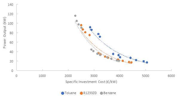
|
The curves follow an exponential relationship and the costs calculated is in good agreement with literature [88]. The majority of the cost of the system according to the methods of Seider et al [44] and Turton et al [43] is in the expander and evaporator/condenser, accounting for almost all the cost of the system. This is in good correlation with the study done by Lecompte et al [50]. For R1233ZD and Benzene, the HEX costs are more than the expander, while for Toluene it is opposite. The study done by Chatzopolou [30], show the variation of cost based on the heat source temperature where the evaporator/condenser is a larger proportion of cost at lower heat source temperatures. However, since the temperatures for this thesis is within fifty degrees, a comparison is not of interest. As expected the recuperated ORC system is cheaper than the simple ORC system as the recuperator decreases the required HEX area significantly and provides a higher power output giving an overall lower SIC.
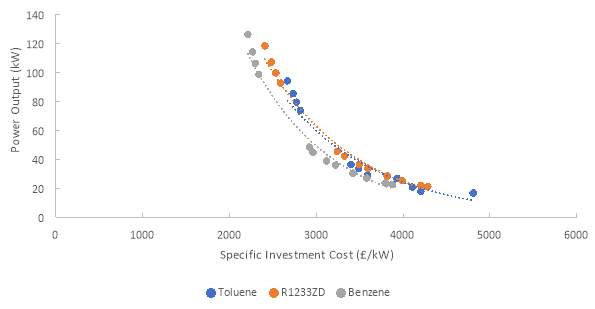
Figure 36 Specific investment cost of recuperated ORC system |
The equations used to calculate the costs do not consider the type of the component. For example, for the expander it can be radial or axial, while HEX types could be plate, shell and tube and tube in tube. The variation of these is not considered, although it is possible to do so by changing the constants. The main difference in cost is in the efficiency of the different types and manufacturing method. One major drawback of this approach is that there is a limit for low capacities and care should be taken at these ranges. At higher capacities, the cost calculated are at the lower end and should not be used as a sole indicator as noted by Chatzopolou [30].
Chapter 5. Concluding Remarks
5.1. Conclusions
This project was undertaken to design a model and evaluate the interaction and performance of one cogeneration combination, a CHP-ORC configuration. At present, there is a real future threat in climate change and there is definite action required. Deploying co-generation systems into commercial buildings is one way of alleviating consumption, by being able to utilise energy more efficiently. There are definite benefits for companies to install CHP units with favourable policies, such as the CHPQA [3], to exempt companies of carbon taxation and decrease fuel consumption to cut cost and emission. It allows companies to supply their own demand during peaks to avoid peak time energy costs. To limit the scope of the problem, the supermarket retail is the sector of choice when considering the demand profile, energy requirements and cost. The supermarket retail sector accounts for 3.5% of the electricity demand in the UK and there is an opportunity to decarbonise the industry.
For this industry, the ICE is one of the most common types of prime movers for the CHP below 1 MW capacity and was chosen because of its reliability, cost, dispatchability and maturity of technology, which are all important criteria for the stakeholder. There is a barrier in coupling the CHP with an ORC system because of a lack of waste heat, but with CHP there is an opportunity to utilise the output heat to get better efficiency and reduced emissions. Different ORC systems were reviewed and compared to select the most suitable type to model. Most of industrial application of ORC systems is geothermal in nature and ORC types associated with geothermal application are not considered. This leaves sub-critical and supercritical ORC systems, but simplicity is preferred and hence a sub-critical ORC system was chosen for this thesis.
To estimate performance and savings more accurately, there is a need to model the integration of the CHP-ORC configuration from first principles, as there is lack of industrial data. To integrate the CHP and ORC, a HEX is used to extract heat from the exhaust gas. A review of HEX types used in literature for integration was performed. Shell and tube heat exchanger was found to be used the most, followed by tube-in tube. In terms of simplicity, tube-in-tube is simpler and was chosen for further examination. For the ORC, the selection of the WF is vital to produce an optimally performing system. There have been many studies investigating the effect of WF’s ranging from low to high temperature application that emphasise the importance of proper WF selection [17, 31, 89]. This thesis deals with high temperature application and WF’s were selected based on a range of criteria including low ODP, GWP, corrosiveness and flammability. Five initial WF’s were chosen, Toluene, R1233ZD, R1234ZE, P-Xylene and Benzene.
The models for the ICE CHP and ORC system were developed by Chatzopolou [11] and was used as a validation tool in the case of the ICE CHP and a sizing tool in the case of the ORC system. The model was used to validate against engines available in the market for CHP-1520, CHP-502 and CHP-310. The results were in good agreement with industrial data, although only 50%, 75% and 100% are specified in the data sheet, the values for 60%, 80% and 90% were estimated. Nonetheless, with the exception of the heat output from the cooling circuit and exhaust gas for CHP-502 and CHP-310, the results were within tolerances specified in the data sheet [73–75], though it might have been at its limit for the two smaller capacities. No further testing was performed to on smaller engines to check for model robustness although it is recommended for future work. The key output used as an input to the ORC system is the exhaust gas mass flow rate and temperature. For CHP-1520, 50-100% part load gave exhaust mass flow ranging from 1.07-2.12 kg/s, while temperature ranges from 420-400 °C. The increase of temperature with part load is a consequence of the engine being less efficient at utilising the fuel at part load.
Two ORC models were used for this thesis, one for a simple ORC system and one that was developed to include a recuperator, giving optimal power output, operating parameters and HEX sizes that is used to determine the part load performance. The ORC system was optimised against 75-100% CHP load because the CHP only operates at full load during peak demand. When the ORC system is optimised against 75% means the ORC system will be operating at 100% and further increase in CHP load would lead to heat being wasted. This might or might not be beneficial depending on supermarket demand and can only be determined through a thermo-economic analysis, which is future work. Of the five initial WF’s, it was narrowed down to three based on power output and efficiency, of which Toluene, R1233ZD and Benzene were found to be most suitable for both simple and recuperated systems. The variation between the two systems are significant. For Toluene, the power output for the simple system ranges from 71.5-91.5 kW depending on CHP part load with an efficiency of 12.1%. This increases for the recuperated system with power output ranging from 73.8-94.2 kW with an efficiency of 14.2%. For R1233ZD, the power output ranges from 75-96 kW for the simple system with an efficiency of 12.6% and 92.6-118.3 kW with an efficiency of 17.3%. For Benzene, these values are 90.5-115.8 kW with an efficiency of 15.2% for the simple system and 98.6-126.2 kW with an efficiency of 17.6%. The benefit of incorporating a recuperator is made clear with these results. R1233ZD sees the highest increase in power and efficiency as it is the only fluid that has significant degree of superheating, having the lowest latent heat of the fluids, giving more recoverable heat than Toluene and Benzene. To get the benefits, the optimiser identified a higher optimal WF mass flow rate to be able to recover more heat. The increased mass flow rate leads to an increase in power output and as the recovered heat is used to preheat the liquid, reduces preheater HEX size. The increase in power output and reduction in extracted heat from exhaust gases gives an increase in efficiency. The differences in power output for the simple system is the gamma value of the fluids, which allows a higher operating pressure ratio for Benzene, while it is similar for Toluene and R1233ZD resulting in similar power output ranges. For the recuperated system, the marked increase in R1233ZD’s power output is a consequence of a significant increase in mass flow rate compared to Toluene and Benzene rather than fluid properties.
The HEX model is developed by Chatzopolou [30] to size the evaporator and condenser. The evaporator is used to extract heat from the exhaust gas while the condenser rejects heat to the environment. The evaporator is divided into three sections, preheater, two-phase evaporator and superheater, while the condenser is divided into desuperheater and two-phase condenser. To size the two-phase evaporator, a few models were used to calculate a mean, because of the complexity associated dealing with two phases. For Toluene, the total evaporator size ranges from 440-513 m2 (75-100% CHP load) for the simple system where the preheater is 86% of the total area. By incorporating a recuperator, 70% of preheater area could be cut and the evaporator size ranges from 150-211 m2. The incorporation of a recuperator gave a substantial benefit to performance and material costs. For R1233ZD and Benzene, the area saving is not as high as Toluene, but still significant, saving 47% and 27% respectively. For R1233ZD, the area ranges from 118-162 m2 for the simple system and 101-140 m2 for the recuperated system. While Benzene have ranges of 206-291 m2 for the simple system and 169-239 m2 for the recuperated system. Toluene differs from R1233ZD and Benzene in one way, the LMTD, giving a much higher area for the simple system. The preheater LMTD of Toluene is much lower than R1233ZD and Benzene, making the heat transfer process much less efficient, requiring more area. The correlation between area and LMTD is quite linear. The condenser area is lower because water is the cooling fluid, which is very effective. The area ranges for Toluene is 1.2-2 m2, 5.6-8.5 m2 for R1233ZD and 2.1-3.1 m2 for Benzene. The fluids display different values depending on mass flow rate or how much of the fluid needs to be cooled. As the mass flow rate of R1233ZD is highest, the condenser area is highest. Toluene has lowest mass flow rate and hence has lowest condenser area.
The part load performance model follows a set of steps to determine the HEX influence on the ORC system. The results of this study indicate that the efficiency increased with part load, because the temperature increase of the exhaust gas played a larger role than the decrease in exhaust mass flow rate. The efficiency for Toluene was observed to range from 15.6%-12.1% (50-100% CHP load) for the simple system and 18.2%-14.2% for the recuperated system. For R1233ZD the efficiency was observed to range from 15.4%-12.1% for the simple system and 23%-17.6% for the recuperated system, while Benzene ranged from 18.6-15.2% for the simple system and 23.2%-17.6% for the recuperated system. The power output still sees a decrease with part load by decreasing the WF mass flow rate, but the net-work drop is proportionally lower than the extracted heat at the evaporator leading to an efficiency increase. The overall heat transfer coefficient was plotted in a graph to compare trends to illustrate the difference of the simple and recuperated system. As the HEX area is fixed for a chosen ORC system, it is the overall heat transfer coefficient that shows the HEX influence of the system and the heat transfer coefficient is dependent on the mass flow rate and temperature. The change in overall heat transfer coefficient was relatively small after an initial drop from full load for both systems. This study helps us understand the HEX interaction of cogeneration systems. Although this study focuses on the HEX influence on the ORC system, it is important to discuss the influence of the pump and expander. In calculating part load performance, the operating points of the system and efficiency of the pump and expander was assumed to be held constant. This is one of the weaknesses of the approach though it can be rectified some. The pump characteristic curve plots mass flow rate against head delivered. As mass flow rate decreases, the pump can deliver more head as it is handling less mass flow. Depending on the pump, the characteristic curve can be steep, large head change with mass flow rate, or flat, small head change with mass flow rate. The mass flow rate change with part load is quite high and in choosing a pump with a flat characteristic curve, aimed to rectify the pump performance variation. In the case of not accounting for the pump variation, the results would have been underestimated, albeit small, as the increased pressure of decreased mass flow rate would only result in a minor change in thermal properties. The expander curve is an efficiency map that considers changes in several parameters. The main parameter in this case is mass flow rate and it deviates away from design point efficiency decreases. When efficiency decreases, the turbine delivers less work in and leads to increased temperature at the turbine outlet, which does, however, lead to more available heat for recovery in the recuperator. The outlet temperature extracted from the model is underestimated and turbine work is overestimated for part load operation. For the expander, the effect of decreased mass flow rate and efficiency compounds leading to worse overall performance.
The SIC methodology for economic analysis is developed by Turton et al [43] and Seider et al [44]. Of the three fluids, Benzene is the cheapest for both systems at 2260 £/kW at 115.8 kW for the simple system and 2200 £/kW at 126.2 kW for the recuperated system. The most expensive is Toluene 5050 £/kW at 16.6 kW for the simple system and 4800 £/kW at 16.7 kW for the recuperated system, while R1233ZD lies in the middle of the SIC range. The cost savings from incorporating a recuperator is the most beneficial for Toluene, saving 250 £/kW at the lower capacity and 102 £/kW at higher capacity. The cost saving is lowest for Benzene, saving 90 £/kW at lower capacity and 60 £/kW at higher capacity. The main weakness with the methodology is not accounting for fluid cost and based purely on system costs. However, it does contrast which is the best performing fluid in terms of sizing. Toluene and Benzene have similar cost per kg, but there is a lack of data for R1233ZD costs. However, since R1233ZD is a relatively new fluid developed for its low GWP and ODP, it is bound to be more expensive and it is possible that it shifts to be more expensive than Toluene overall. One major drawback of this approach is that there is a limit for low capacities and care should be taken at these ranges. At higher capacities, the cost calculated are at the lower end and should not be used as a sole indicator as noted by Chatzopolou [30].
A limitation of this study is that the behaviour found from the modelling will be applicable to ICE CHP, sub-critical ORC, tube-in-tube HEX and pumps with flat characteristic curves only. Despite the limited application, this study manages to give a framework and will be able to expand the technology base in the future.
5.2. Recommendation for future work
The TSO model is a techno-economic mixed integer linear programming model that function as a decision-making tool for optimal selection and operation of energy systems. Figure 37 shows the interaction and process diagram on how the model functions. There are currently some restrictions with the model that needs to be rectified to get optimal output. To achieve optimisation of the linear model requires linear inputs to be fed into the model. The TSO model is as presented by Cedillos [79], giving an overview of its capabilities. The TSO model is the adopted method to be used for optimisation using linear programming to achieve its goals. The model has many built in capabilities, given energy demands profiles and location to determine fuel and energy costs, technologies with associated capacities, costs and efficiencies. Additionally, it puts a price on energy and emissions to fully cover the whole scope of determining the best solutions. From these parameters, the model has an objective to minimise cost, GHG emission or a combination of both. Since the model can consider demand of timed intervals, the general profile is also required. It is also possible to set the level of load of the technologies ranging from 50-100%. This is included to simulate part load operations, although it is currently assuming constant efficiency for part load. Part of the objective was to simulate the part load performance to get more accurate outcomes. With the HEX influence determined, future work should aim towards modelling the influence of the pump and expander to capture the full part load performance constituents. Additionally, the model should be expanded to encompass all types of HEX’s, pumps and expanders to get a full grasp on which technology is most suitable for different applications and power output ranges.
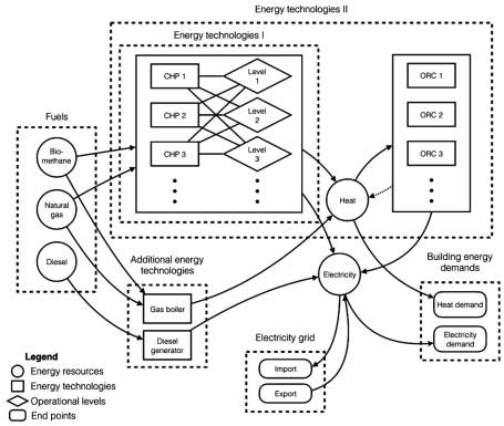
|
Chapter 6. References
[1] International Energy Agency (IEA), “Key world energy trends – excerpt from: world energy balances,” Iea, p. 19, 2016.
[2] Department for Bussiness Energy & Industrial Stratergy, “Energy Consumption,” Crown Copyr., no. July, 2016.
[3] DECC, “The CHPQA Standard,” Chpqa, no. 1, p. 18, 2013.
[4] Ofgem, “Demand side response in the non-domestic sector,” no. May, pp. 1–65, 2012.
[5] S. Acha, “Challenges in Decarbonising Commercial Real Estate in the UK,” no. January, 2017.
[6] T. C. Wagner, “Energy-Savings Systems for Commercial Building CHP and Industrial Waste Heat Applications,” Cogener. Distrib. Gener. J., vol. 19, no. 4, pp. 66–80, 2004.
[7] N. Sugiartha, S. A. Tassou, I. Chaer, and D. Marriott, “Trigeneration in food retail: An energetic, economic and environmental evaluation for a supermarket application,” Appl. Therm. Eng., vol. 29, no. 13, pp. 2624–2632, 2009.
[8] S. Murugan and B. Horák, “Tri and polygeneration systems – A review,” Renew. Sustain. Energy Rev., vol. 60, pp. 1032–1051, 2016.
[9] H. Al Moussawi, F. Fardoun, and H. Louahlia-Gualous, “Review of tri-generation technologies: Design evaluation, optimization, decision-making, and selection approach,” Energy Convers. Manag., vol. 120, pp. 157–196, 2016.
[10] V. Vukašinović, D. Gordić, M. Babić, D. Jelić, and D. Končalović, “Review of efficiencies of cogeneration units using internal combustion engines,” Int. J. Green Energy, vol. 13, no. 5, pp. 446–453, 2016.
[11] M. A. Chatzopoulou and C. N. Markides, “Modelling of Advanced Combined Heat and Power Systems,” Astfe 2017, pp. 1–16, 2017.
[12] Y. A. Cengel and M. A. Boles, Thermodynamics: an Engineering Approach 8th Edition. 2015.
[13] H. Cho, R. Luck, and L. M. Chamra, “Imece2009-11634 Power Generation and Heat Recovery Model of Reciprocating,” pp. 1–7, 2009.
[14] U. S. E. P. Agency, C. Heat, and P. P. Chp, “Section 2 . Technology Characterization – Reciprocating Internal Combustion Engines,” Cat. CHP Technol., no. March, 2015.
[15] U. States Department of Energy, “Combined Heat and Power Technology Fact Sheet Series: Microturbines,” pp. 2–5, 2015.
[16] K. Rahbar, S. Mahmoud, R. K. Al-Dadah, N. Moazami, and S. A. Mirhadizadeh, “Review of organic Rankine cycle for small-scale applications,” Energy Convers. Manag., vol. 134, pp. 135–155, 2017.
[17] H. Chen, D. Y. Goswami, and E. K. Stefanakos, “A review of thermodynamic cycles and working fluids for the conversion of low-grade heat,” Renew. Sustain. Energy Rev., vol. 14, no. 9, pp. 3059–3067, 2010.
[18] D. Mikielewicz and J. Mikielewicz, “A thermodynamic criterion for selection of working fluid for subcritical and supercritical domestic micro CHP,” Appl. Therm. Eng., vol. 30, no. 16, pp. 2357–2362, 2010.
[19] S. Lecompte, H. Huisseune, M. Van Den Broek, B. Vanslambrouck, and M. De Paepe, “Review of organic Rankine cycle (ORC) architectures for waste heat recovery,” Renew. Sustain. Energy Rev., vol. 47, pp. 448–461, 2015.
[20] X.-R. Zhang, H. Yamaguchi, and D. Uneno, “Experimental study on the performance of solar Rankine system using supercritical CO2,” Renew. Energy, vol. 32, no. 15, pp. 2617–2628, 2007.
[21] C. Wieland, D. Meinel, S. Eyerer, and H. Spliethoff, “Innovative CHP concept for ORC and its benefit compared to conventional concepts,” Appl. Energy, vol. 183, pp. 478–490, 2016.
[22] D. Ziviani, A. Beyene, and M. Venturini, “Advances and challenges in ORC systems modeling for low grade thermal energy recovery,” Appl. Energy, vol. 121, pp. 79–95, 2014.
[23] B. T. Liu, K. H. Chien, and C. C. Wang, “Effect of working fluids on organic Rankine cycle for waste heat recovery,” Energy, vol. 29, no. 8, pp. 1207–1217, 2004.
[24] A. Javanshir and N. Sarunac, “Thermodynamic analysis of a simple Organic Rankine Cycle,” Energy, vol. 118, pp. 85–96, 2017.
[25] W. Sun, X. Yue, and Y. Wang, “Exergy efficiency analysis of ORC (Organic Rankine Cycle) and ORC-based combined cycles driven by low-temperature waste heat,” Energy Convers. Manag., vol. 135, pp. 63–73, 2017.
[26] N. F. Tumen Ozdil, M. R. Segmen, and A. Tantekin, “Thermodynamic analysis of an Organic Rankine Cycle (ORC) based on industrial data,” Appl. Therm. Eng., vol. 91, pp. 43–52, 2015.
[27] G. Cavazzini and P. Dal Toso, “Techno-economic feasibility study of the integration of a commercial small-scale ORC in a real case study,” Energy Convers. Manag., vol. 99, pp. 161–175, 2015.
[28] O. Dumont, “Modelling of organic Rankine cycle power systems in off-design conditions : An experimentally-validated comparative study,” vol. 123, 2017.
[29] F. A. Al-sulaiman, I. Dincer, and F. Hamdullahpur, “Thermoeconomic optimization of three trigeneration systems using organic Rankine cycles : Part I – Formulations,” Energy Convers. Manag., vol. 69, pp. 199–208, 2013.
[30] Chatzopoulou and C. N. Markides, “Thermoeconomic Analysis of ORC : Equipment Sizing Methods.”
[31] N. A. Lai, M. Wendland, and J. Fischer, “Working fluids for high-temperature organic Rankine cycles,” Energy, vol. 36, no. 1, pp. 199–211, 2011.
[32] J. Larjola, “Electricity from industrial waste heat using high-speed organic Rankine cycle (ORC),” Int. J. Prod. Econ., vol. 41, no. 1–3, pp. 227–235, 1995.
[33] I. Obernberger, P. Thonhofer, and E. Reisenhofer, “Description and evaluation of the new 1,000 kWel Organic Rankine Cycle process integrated in the biomass CHP plant in Lienz, Austria,” Euroheat & Power, vol. 10, pp. 1–17, 2002.
[34] U. Drescher and D. Br??ggemann, “Fluid selection for the Organic Rankine Cycle (ORC) in biomass power and heat plants,” Appl. Therm. Eng., vol. 27, no. 1, pp. 223–228, 2007.
[35] EC, “EU F-Gas Regulation Guidance Information Sheet 26 : Bans for New Products and Equipment Target audience for this Information Sheet New Products and Equipment : F-Gas Ban Summary Table,” no. December 2014, pp. 1–3, 2015.
[36] Linde Gases Division, “Guide to updated EU f-gas regulation (517/2014),” no. July, pp. 1–32, 2014.
[37] H. Brown, “Reducing the impact of climate change.,” Bull. World Health Organ., vol. 85, no. 11, pp. 824–825, 2007.
[38] T. C. Hung, S. K. Wang, C. H. Kuo, B. S. Pei, and K. F. Tsai, “A study of organic working fluids on system efficiency of an ORC using low-grade energy sources,” Energy, vol. 35, no. 3, pp. 1403–1411, 2010.
[39] J. Bao and L. Zhao, “A review of working fluid and expander selections for organic Rankine cycle,” Renew. Sustain. Energy Rev., vol. 24, pp. 325–342, 2013.
[40] L. O. W. G. W. P. Hydrofluoroolefins, “The environmental alternative to traditional refrigerants Fourth Generation Refrigerants for the 21st Century Solstice ze Refrigerant.”
[41] K. Gluesenkamp, Y. Hwang, and R. Radermacher, “High efficiency micro trigeneration systems,” Appl. Therm. Eng., vol. 50, no. 2, pp. 1480–1486, 2013.
[42] J. P. Roy, M. K. Mishra, and A. Misra, “Performance analysis of an Organic Rankine Cycle with superheating under different heat source temperature conditions,” Appl. Energy, vol. 88, no. 9, pp. 2995–3004, 2011.
[43] R. Turton, R. C. Bailie, W. B. Whiting, J. A. Shaeiwitz, and D. Bhattacharyya, Analysis, Synthesis, and Design of Chemical Processes, vol. 53, no. 9. 2012.
[44] W. D. Seider, J. D. Seader, and D. R. Lewin, Product & Process Design Principles – Synthesis, Analysis & Evaluation. 2003.
[45] A. K. Hueffed, “Analysis and optmization of CHP, CCHP, CHP-ORC, and CCHP-ORC systems,” ProQuest Diss. Theses, no. May, p. 161, 2010.
[46] P. J. Mago, A. Hueffed, and L. M. Chamra, “Analysis and optimization of the use of CHP-ORC systems for small commercial buildings,” Energy Build., vol. 42, no. 9, pp. 1491–1498, 2010.
[47] Q. Zhu, Z. Sun, and J. Zhou, “Performance analysis of organic rankine cycles using different working fluids,” Therm. Sci., vol. 19, no. 1, pp. 179–191, 2015.
[48] A. P. Marantan, “Optimization of integrated microturbine and absorption chiller systems in CHP for buildings applications,” p. 112, 2002.
[49] T. a Ibrahim, “THE DEVELOPMENT OF AN AIR-COOLED ABSORPTION CHILLER CONCEPT AND ITS INTEGRATION IN CHP SYSTEMS Xiaohong,” System, vol. d, no. Chapter 6, 2003.
[50] S. Lecompte, H. Huisseune, M. van den Broek, S. De Schampheleire, and M. De Paepe, “Part load based thermo-economic optimization of the Organic Rankine Cycle (ORC) applied to a combined heat and power (CHP) system,” Appl. Energy, vol. 111, pp. 871–881, 2013.
[51] S. Quoilin, M. Van Den Broek, S. Declaye, P. Dewallef, and V. Lemort, “Techno-economic survey of organic rankine cycle (ORC) systems,” Renew. Sustain. Energy Rev., vol. 22, pp. 168–186, 2013.
[52] H. C. Jung and S. Krumdieck, “Modelling of organic Rankine cycle system and heat exchanger components,” Int. J. Sustain. Energy, vol. 33, no. 3, pp. 704–721, 2014.
[53] C. Zhang, C. Liu, S. Wang, X. Xu, and Q. Li, “Thermo-economic comparison of subcritical organic Rankine cycle based on different heat exchanger configurations,” Energy, vol. 123, pp. 728–741, 2017.
[54] R. Mastrullo, A. W. Mauro, R. Revellin, and L. Viscito, “Modeling and optimization of a shell and louvered fin mini-tubes heat exchanger in an ORC powered by an internal combustion engine,” Energy Convers. Manag., vol. 101, pp. 697–712, 2015.
[55] S. Karellas, A. Schuster, and A. D. Leontaritis, “Influence of supercritical ORC parameters on plate heat exchanger design,” Appl. Therm. Eng., vol. 33–34, no. 1, pp. 70–76, 2012.
[56] O. Oyewunmi and C. Markides, “Thermo-Economic and Heat Transfer Optimization of Working-Fluid Mixtures in a Low-Temperature Organic Rankine Cycle System,” Energies, vol. 9, no. 6, p. 448, 2016.
[57] M. Anna and C. N. Markides, “Advancements in Organic Rankine Cycle System Optimisation for Combined Heat and Power Applications : Components Sizing and Thermoeconomic Considerations,” 2017.
[58] The Mathworks Inc., “MATLAB – MathWorks,” www.mathworks.com/products/matlab, 2016. [Online]. Available: http://www.mathworks.com/products/matlab/.
[59] E. W. W. Lemmon, M. L. L. Huber, and M. O. O. McLinden, “NIST Standard Reference Database 23: Reference Fluid Thermodynamic and Transport Properties (REFPROP), Version 9.0,” Phys. Chem. Prop. …, 2010.
[60] J. I. Ghojel, “Review of the development and applications of the Wiebe function: A tribute to the contribution of Ivan Wiebe to engine research,” Int. J. Engine Res., vol. 11, no. 4, pp. 297–312, 2010.
[61] K. T. Yun, H. Cho, R. Luck, and P. J. Mago, “Modeling of reciprocating internal combustion engines for power generation and heat recovery,” Appl. Energy, vol. 102, pp. 327–335, 2013.
[62] P. K. Kundu, Compressible Flow. 2012.
[63] J. Nouman, “Comparative studies and analyses of working fluids for Organic Rankine Cycles – ORC,” 2012.
[64] F. P. Incropera, T. L. Bergman, A. S. Lavine, and D. P. DeWitt, Fundamentals of Heat and Mass Transfer. 2011.
[65] V. Gnielinski, “New Equations for Heat and Mass Transfer in Turbulent Pipe and Channel Flow,” Int. Chem. Eng., vol. 16, no. 2, pp. 359–368, 1976.
[66] J. R. Garc??a-Cascales, F. Vera-Garc??a, J. M. Corber??n-Salvador, J. Gonz??lvez-Maci??, and D. Fuentes-D??az, “Assessment of boiling heat transfer correlations in the modelling of fin and tube heat exchangers,” Int. J. Refrig., vol. 30, no. 6, pp. 1004–1017, 2007.
[67] J. C. Dobson, M.K, Wattelet, J.P, Chato, “Optimal Sizing of Two-Phase Heat Exchangers,” 1993.
[68] T. R. Hewitt, G.F, Shires, GL, Bott, “Process heat transfer,” CRC Press, 1994.
[69] V. D. I. V., “VDA Heat Atlas,” Springer, vol. 2, no. 2, 2010.
[70] M. M. Shah, “A general correlation for heat transfer during film condensation inside pipes,” Int. J. Heat Mass Transf., vol. 22, no. 4, pp. 547–556, 1979.
[71] F. Calise, C. Capuozzo, A. Carotenuto, and L. Vanoli, “Thermoeconomic analysis and off-design performance of an organic Rankine cycle powered by medium-temperature heat sources,” Sol. Energy, vol. 103, pp. 595–609, 2014.
[72] Chemengonline, “CEPCI June 2017 Issue.” [Online]. Available: https://www.scribd.com/document/352561651/CEPCI-June-2017-Issue.
[73] Ener-G, “E1520 500NOx L64 Natural Gas CHP Unit,” p. 7457, 2014.
[74] Ener-G, “E530M Natural Gas CHP Unit Datasheet,” p. 7457, 2015.
[75] Ener-G, “E310M Natural Gas CHP Unit Datasheet,” p. 7457, 2015.
[76] A. Cairns, A. Todd, P. Aleiferis, and J. Malcolm, “A comparison of inlet valve operating strategies in a single cylinder spark ignition engine.”
[77] T. C. Hung, “98/01752 A review of organic Rankine cycles (ORCs) for the recovery of low-grade waste heat: Hung, T. C. et al. Energy, 1997, 22, (7), 661–667,” Fuel Energy Abstr., vol. 39, no. 2, p. 151-, 1998.
[78] P. J. Mago, L. M. Chamra, K. Srinivasan, and C. Somayaji, “An examination of regenerative organic Rankine cycles using dry fluids,” Appl. Therm. Eng., vol. 28, no. 8–9, pp. 998–1007, 2008.
[79] D. Cedillos Alvarado, S. Acha, N. Shah, and C. N. Markides, “A Technology Selection and Operation (TSO) optimisation model for distributed energy systems: Mathematical formulation and case study,” Appl. Energy, vol. 180, pp. 491–503, 2016.
[80] S. Mariaud, A, Acha, “CHP_spreadsheet.” 2016.
[81] KSB, Selecting Centrifugal Pumps. 2005.
[82] Y. Q. Feng et al., “Operation characteristic of a R123-based organic Rankine cycle depending on working fluid mass flow rates and heat source temperatures,” Energy Convers. Manag., vol. 131, pp. 55–68, 2017.
[83] G. Qiu, H. Liu, and S. Riffat, “Expanders for micro-CHP systems with organic Rankine cycle,” Appl. Therm. Eng., vol. 31, no. 16, pp. 3301–3307, 2011.
[84] X. Yang, J. Xu, Z. Miao, J. Zou, and C. Yu, “Operation of an organic Rankine cycle dependent on pumping flow rates and expander torques,” Energy, vol. 90, pp. 864–878, 2015.
[85] T. Deka, “‘ Analytical study of a Turbo-charging Device ,’” no. September, 2015.
[86] Platts, “PLATTS GLOBAL TOLUENE PRICE INDEX.” [Online]. Available: https://www.platts.com/news-feature/2014/petrochemicals/pgpi/toluene. [Accessed: 22-Aug-2017].
[87] Platts, “PLATTS GLOBAL BENZENE PRICE INDEX.” [Online]. Available: https://www.platts.com/news-feature/2014/petrochemicals/pgpi/benzene. [Accessed: 22-Aug-2017].
[88] S. Lemmens, “Cost engineering techniques and their applicability for cost estimation of organic rankine cycle systems,” Energies, vol. 9, no. 7, 2016.
[89] F. Ayachi, E. Boulawz Ksayer, A. Zoughaib, and P. Neveu, “ORC optimization for medium grade heat recovery,” Energy, vol. 68, pp. 47–56, 2014.
Cite This Work
To export a reference to this article please select a referencing stye below:
Related Services
View all


Related Content
All TagsContent relating to: "Energy"
Energy regards the power derived from a fuel source such as electricity or gas that can do work such as provide light or heat. Energy sources can be non-renewable such as fossil fuels or nuclear, or renewable such as solar, wind, hydro or geothermal. Renewable energies are also known as green energy with reference to the environmental benefits they provide.
Related Articles

DMCA / Removal Request
If you are the original writer of this dissertation and no longer wish to have your work published on the UKDiss.com website then please: