1.1         Problem Description

The proposed mathematical model extends the research done by Zeng et al. (2017) with the objective of minimizing the total cost. The model handles a transshipment hub terminal which is visited by both feeder and mother vessels with estimated arrival times and specific containers capacity.

1.1.1        Transshipment and Non-Transshipment Containers

The incoming vessels might have containers to be transshipped to another vessel arriving at the terminal within the predetermined planning horizon. These transshipment containers might be unloaded and transferred to the yard storage area for some time before being loaded onto another vessel. Alternatively, the calling schedule for both vessels can be adjusted so that the containers can be directly transshipped. One of the most important features of the proposed mathematical model is to counteract this situation and decide the transshipment method that should be used for each pair of vessels individually by comparing the associated total cost of both scenarios.

In addition to transshipment containers, vessels might have other non-transshipment operations exchanged with the terminal yard area and considered as import/export containers as suggested by Liang et al. (2012). Unloaded containers might leave the terminal either by being loaded to another vessel arriving after the specified planning horizon or by leaving through the terminal gate. Loaded containers could come to the terminal from its gate or could be dropped by a previously arrived vessel. However, handling sources and sinks of those non-transshipment containers are beyond the scope of this study.

1.1.2        Representation of Vessels Service Order

For instance, consider feeder vessel

jwhich has containers to be transshipped to mother vessels

iand

gin addition to the non-transshipment containers. Thus, there are three possible service orders for feeder vessel

j while each operation can be handled at any order. As an example, the non-transshipment containers can be handled at the first, second, or even the third service order. The only requirement to be considered is to finish handling all containers included at a specific operation before working on the following one.

One of the possible scenarios for feeder vessel

jservice order is as follows with a graphic representation shown at Figure 5:

• First, unload containers for mother vessel

  g(1^st service order)

• Then, handle non-transshipment containers (2^nd service order)
• Finally, unload containers for mother vessel

  i(3^rd service order)

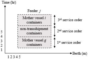
Figure 5. Feeder vessel j service order possible sequence (a)

As illustrated in Figure 5, the vessel is represented by a rectangle with a horizontal dimension equal to its length and a vertical dimension expressing berthing time (Meisel and Bierwirth, 2006). Each bordered box within the vessel rectangle indicates the start and end times of each handling operation. Figure 6 shows another feasible scenario for the same feeder vessel:

• First, handle non-transshipment containers (1^st service order)
• Then, unload containers for mother vessel

  g(2^nd service order)

• Finally, unload containers for vessel

  i(3^rd service order)

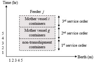
Figure 6. Feeder vessel j service order possible sequence (b)

The concept of “service order” has been commonly addressed in literature (see Imai et al., 2001). Container terminals studied in most of these research papers have a specified number of discrete berths. Since each berth can only accommodate one vessel at a time, vessels arriving at the terminal need to be allocated to those berths with a service order that guarantees no overlapping between vessels at the same berth. The same concept is applied on vessels that have transshipment relationship with other vessels. In this research, an optimization model is proposed to handle this critical decision. The proposed model employs a mixed integer linear program (MILP) and focuses on the dynamic nature of how berth allocation planning and sequencing of service orders may be co-handled by adjusting transshipment operation schedule. As soon as a transshipment method is chosen, the model generates service orders for vessels that minimizes total turnaround time of vessels and the associated waiting cost.

1.1.3        Berth Allocation Planning and Sequencing of Service Orders

Berth allocation assigns berthing position and berthing time for incoming feeders and mother vessels along the terminal quay. The next sections explain each problem individually in detail.

• Berthing Position Allocation:

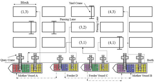
The model assigns a berthing location while maintaining minimum total travel distance for both non-transshipment and transshipment containers. Non-transshipment containers move from quayside area to the assigned yard blocks. As shown in Figure 7, import containers are unloaded from mother vessels and transported to the designated yard blocks. Similarly, feeder vessels load export containers from yard blocks. Meanwhile, travelled distance for transshipment containers is determined according to the transshipment method chosen by the model, which will be either direct or traditional. By applying the traditional method, containers arrive and depart on vessels while being temporarily stored in the yard (Giallombardo, et al., 2010), such as the non-transshipment containers. The vessel must be allocated to a berthing position close enough to the designated yard blocks in order to speed up the vessel handling time. An example of the service flow for the indirect-transshipment containers case is shown in Figure 7, where the transshipment containers for mother vessel A will be discharged from feeder vessel C and stored at the designated yard block. Once mother vessel A is ready for the loading process, containers will be loaded to it. However, for the direct-transshipment case, containers are transferred from one vessel to another directly. Transferring containers from feeder D to mother vessels A and B is an example of a direct-transshipment case (see Figure 7).

The proposed model allocates a berthing position for each incoming vessel in such a way that minimizes the overall travelled distance for all containers. It is worthwhile to mention that each group of containers is assigned randomly to a yard block within the terminal. In other words, yard block assignment is an input parameter not a decision variable. For the example shown in Figure 7, if containers from feeder C to mother vessel A are transshipped through the terminal, they will be stored at yard block (3,1). Note that two decision variables are generated randomly by the proposed model; berthing positions along the quay and the transshipment method. Accordingly, the travelled distances as well as the incorporated costs are calculated based on model constraints and assumptions. The following input parameters determine the terminal layout dimensions and contribute to the distance calculations (Readers are referred to Chapter 4 for more detailed information):

• yard block length and width
• passing lane width
• horizontal distance between yard blocks,
• distance between quayside area to yard-side area

Figure 7. Transshipment Terminal Layout Legend:
	Transshipment containers from Feeder D to mother vessel A
	Transshipment containers from Feeder C to mother vessel A
	Import and Export containers for vessels A, B, C, and D
	Transshipment containers from Feeder D to mother vessel B
	Transshipment containers from Feeder C to mother vessel B
	Flow for indirect transshipment containers
	Flow for import and export containers (non-transshipment)
	Flow for direct transshipment containers

• Berthing Time Determination:

The former example is used to illustrate how vessel’s berthing time mainly depends on the decided transshipment method. Table 3 lists the handling operations related to each vessel individually

Table 3. Vessels handling operations

Item	Operation	Schedule
Mother vessel g	Containers from feeder vessel j Non-transshipment containers	Arrival time: ag Service orders: 2
Mother vessel i	Containers from feeder vessel j Non-transshipment containers	Arrival time: ai Service orders: 2
Feeder vessel j	Containers for mother vessel g Containers for mother vessel i Non-transshipment containers	Arrival time: aj Service orders: 3

Containers might be transshipped from feeder

jto both mother vessels

gand

iusing direct or traditional method at any service order. It is important to note that, the decision to transfer containers from vessel

jto vessel

gusing the direct transshipment method, does not strictly require vessel

jto transfer containers to vessel

idirectly as well, since the transshipment method is decided for each pair of vessels {(j, g) and (j, i)} separately. All possible scenarios for this example are shown in Figure 8.

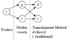
Figure 8. Possible transshipment scenarios

Scenario (1):  Feeder

j, mother vessel

g- direct transshipment

Feeder

j, mother vessel

i  – direct transshipment

To directly transfer containers between vessels (

j,

g), both vessels should be arrived at the terminal and allocated to different berthing positions. Vessels also should be idle and not busy working with other containers to be able to start the handling operation between them. As can be seen in Figure 9, mother vessel

gwaits for feeder

jto finish its non-transshipment operation, then containers are unloaded from feeder

jand transferred to vessel

gberthing position. Vessels (

j,

i) are treated in exactly the same manner to directly exchange containers between them. Figure 9 also highlights an important issue to discuss, i.e., containers transshipped between two vessels do not have to be handled at the same service order from each vessel perspective. Containers between vessels (

j,

g) are handled at feeder

j’s 2^nd service order while mother vessel

gis at its 1^st service order. It’s only worthwhile to accurately manage berthing time of both vessels, as stated earlier. Similar to Figure 5, each rectangle in Figure 9 represents the Berthing schedule of a vessel. The positions of the horizontal sides represent the Berthing locations, while the lengths of the horizontal sides correspond to the lengths of the corresponding vessels. Also, the position of a vertical side corresponds to the duration from the starting to the ending time of the operation of a vessel, while the dotted lines are the arrival times to that port (Park and Kim, 2005).

Therefore, there are many possible combinations for scenario (1), which can be generated by changing the sequence of service orders for each vessel. Each sub-scenario results in different waiting time for vessels. One of these combinations is represented at Figure 10, which shows a different service order for feeder

j. It is notable that the waiting time pattern and value for each vessel has changed from the former scenario (1a). Feeder vessel

jwaits for both mother vessels which have no waiting time. This discussion aims at enforcing the importance of service orders and illustrating how different combinations can impact on the total turnaround time of vessels.

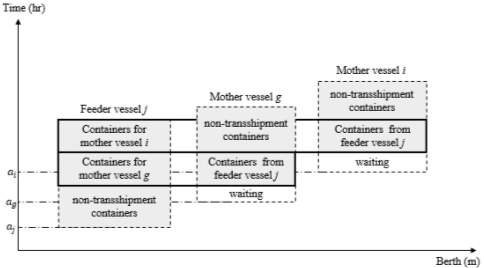
Figure 9. Berth plan for Scenario (1a) – direct transshipment

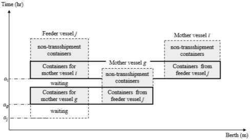
Figure 10. Berth plan for Scenario (1b) – direct transshipment

Scenario (2):  Feeder

j, mother vessel

g- direct transshipment

Feeder

j, mother vessel

i  – traditional transshipment

In this scenario, containers between vessels (

j,

g) are exchanged similar to the one illustrated in Figure 9. The only difference between scenario (1a) and (2a), is on the transshipment method for transferring containers from feeder

jto mother vessel

i. At the traditional transshipment configuration, containers should be already unloaded from feeder

jto the storage yard, and then loaded onto mother vessel

i. As shown in Figure 11, mother vessel

ihas a longer waiting time as a result of the sequenced service orders along with determined transshipment method. Another service order sequence related to mother vessels

iis illustrated in Figure 12, where it starts the unloading/loading operations of non-transshipment containers once being assigned to a berth position. This configuration minimizes the total waiting time of vessel. Other relationships between vessels can be interpreted easily by the same way (see Figure 12).

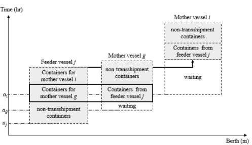
Figure 11. Berth plan for Scenario (2a) – direct/traditional transshipment

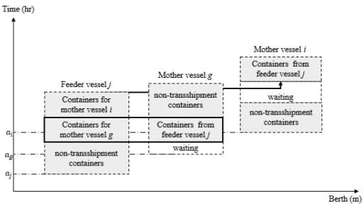
Figure 12. Berth plan for Scenario (2b) – direct/traditional transshipment

To summarize what’s been mentioned so far, vessels may need to wait for each other, regardless of the decided transshipment method. This waiting time may occur before the start of handling operations or even between service orders. Hence, proper sequencing of service orders certainly defines vessels berthing time and minimizes the total undesirable waiting time of incoming vessels.

1.1.4        Model Assumptions: (Omnia, please provide a rational for each assumption)

• Relationship between vessels occurs only between feeders and mother vessels with predetermined capacity that flows from feeders to mother vessels
• Transshipments can be conducted between many vessels at the same time. Thus, mother vessels can be associated with six feeders at most, while feeders can be assigned up to three mother vessels
• Containers between vessels can be transshipped by using either traditional or direct transshipment methods
• Incoming vessels can berth anywhere along the quay with no physical restrictions
• Feeder and mother vessels have known capacity of non-transshipment containers which can be handled at any service order
• Estimated arrival times for incoming vessels and storage yard blocks for containers are predetermined

1.2         Problem Formulation

The proposed optimization model employs a mixed integer linear program (MILP) and focuses on finding berthing positions, determining transshipment method, developing sequence of service orders, and assigning starting time of each handling operation. The notation used throughout this thesis is stated below:

1.2.1        Sets

I	Mother vessels (1…, b)
J	Feeder vessels (b+1…, e)
K	Service orders (1…, l) Note that, each vessel has different number of service orders, which is the number of other vessels that has transshipment relationship with it, in addition to one more service order for the vessel’s non-transshipment containers.
m	Blocks at the parallel direction of the quay (1…, g)
n	Blocks at the perpendicular direction of the quay (1…, f)
φj	Set of mother vessels that have transshipment containers with feeder j. Note that there is hjnumber of mother vessels at φj
φi	Set of feeders that have transshipment containers with mother i.There is hinumber of feeders at φi
∂j	Set of service orders assigned to each feeder j. Number of service orders at ∂jis pj=hj+1
∂i	Set of service orders assigned to each mother vessel i. Number of service orders at ∂iis pi=hi+1

1.2.2        Parameters

L	The port quay length
li	Vessels length, ∀ i∈I∪J
TCji	Transshipment containers between feeder vessel jand mother vessel i
TTji	The time required to handle transshipment containers between feeder jand mother vessel i, which depends on number of TCji,number of assigned quay cranes, and the working speed of QCs TTji=TCjiδ.γ
δ	Working speed of QCs, it is assumed to be 40TEU/h based on (Liang et al.,2012)
γ	Number of QCs, it is assumed that there is one quay crane assigned to each vessel
NTi	Non-transshipment containers assigned to each vessel, ∀ i∈I∪J
NTTi	The time required to finish working with non-transshipment containers for each vessel, ∀ i∈I∪J
ai	Scheduled arrival time for vessels, ∀ i∈I∪J
hi	Number of vessels that has transshipment relationship with vessel i, ∀ i∈I∪J
pi	Number of service orders attached vessel i, ∀ i∈I∪J
Vimn	1: If non-transshipment containers assigned to m and n yard block ∀i∈I∪J, ∀ m∈M, ∀ n∈N 0: otherwise
Vijmn	1: If transshipment containers between iand jvessels are assigned to mand nyard block ∀i∈I,  j∈φi,  ∀ m∈M,  ∀ n∈N 0: otherwise
α	Block yard length
β	Block yard width
d	Travelled distance from quay side area to the yard side area
M	Sufficient large constant
c1	Transport cost of yard trailers (USD/m*TEU)
c2i	Penalty cost of vessel idue to the delay of berth allocation from the vessel arrival time, in addition to vessel i’s waiting time for other vessels to perform direct transshipment operation (USD/h)
c3	Handling cost of yard cranes (USD/TEU)

1.2.3        Decision Variables

xi	Berthing position of vessels, ∀ i∈I∪J
Sijk	Starting time of vessel ito handle the transshipment containers with vessel jat kth service order ∀ k∈∂i, ∀ i,j∈I∪J, i≠j
yijk	1: if vessel ihandles the transshipment containers with vessel jat kth service order ∀ k∈∂i, ∀ i,j∈I∪J 0: otherwise
Sik	Starting time of vessel ito handle non-transshipment containers at kth service order, ∀ k∈∂i and i∈I∪J
yik	1: if vessel ihandles non-transshipment containers at kth service order, ∀ k∈∂i and i∈I∪J 0: otherwise
Aji	0: if transshipment containers are transferred from feeder jto mother vessel idirectly 1: otherwise
Zji	1: if vessel jberthing position is to the left of vessel ilocation 0: otherwise
Bji	1: if vessel jscheduled to berth before vessel i 0: otherwise

Note that, there is no mentioned decision variable that determines the berthing time for each vessel, in the previous section. This is because the vessel’s berthing time has the same start time of the handling operation assigned at the first job. Therefore, the berthing time of feeder

jat the example shown in Figure 13 is equal to

Sjg1. It is also important to note that decision variables

Sijkrepresenting the start time for each incoming vessel depends on its transshipment relationship with other vessels. For instance, feeder

jat Figure 13 has two transshipment flows with mother vessels

iand

g. Consequently, the mathematical model generates two decision variables for feeder

j, which are

Sjikand

Sjgk, in addition to the starting time variable for related non-transshipment containers

Sjk. Moreover, vessels depart the terminal as soon as the last handling job has finished. For the example considered at Figure 13, the finishing time for feeder

j’s berthing can be calculated as

(Sji3+TTji).

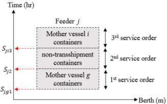
Figure 13. starting times of handling operations for feeder j

1.2.4        Mathematical Model

The objective function of the proposed model minimizes the total transportation and handling costs for both non-transshipment and transshipment containers with five different components. The first two components (1.1 and 1.2) are the penalty cost for feeder and mother vessels respectively. The cost is calculated based on the waiting time for each vessel between its arrival and departure times. Component (1.3) is the transport cost for yard trucks while handling vessels’ non-transshipment containers. It is worthwhile to note that this cost is affected by the allocated berth position for each vessel. Meanwhile, yard trucks transport cost for transshipment containers is determined at component (1.4). For direct transshipment case, the trucks move back-and-forth between berth positions of two vessels. However, for traditional transshipment case, yard trucks pick up containers from feeder vessel berth location to yard blocks, and then drop them into mother vessel location. Component (1.5) represents yard gantry crane cost while handling transshipment containers when using the traditional method (

Aji=1).

Min	∑j∈Jc2j∑i∈φj  ∑k∈∂j|k=pjSijkYijk+∑k∈∂j|k=pjSjkYjk-aj-∑i∈φj  ∑k∈∂j|k<pjTTjiYijk-∑k∈∂j|k<pjNTTjYjk
	+∑i∈Ic2i∑j∈φi  ∑k∈∂i|k=piSijkYijk+∑k∈∂i|k=piSikYik-ai-∑j∈φi  ∑k∈∂i|k<piTTjiYijk-∑k∈∂i|k<piNTTiYik
	+∑i∈I∪J∑m∈M∑n∈Nc1NTTiVimnα*m-xi+β*n+d
	+∑i∈I∑j∈φi∑m∈M∑n∈Nc1TCjiVjimn[Ajiα*m-xj+β*n+d+1-Ajixi-xj+Ajiα*m-xi+β*n+d]
	+∑i∈I∑j∈φic3(TCjiAji)

Subject to various constraints as follows:

1. The first constraint indicates that transshipment containers between two vessels must be handled only once for any vessels

∑k∈∂iYijk=1,  ∀ i∈I∪J,  ∀ j∈φi

2. The constraint (3) ensures that incoming vessels must work with only one handling operation including non-transshipment or transshipment containers at the same service order

∑j∈φiYijk+Yik=1,  ∀ i∈I∪J,  ∀ k∈∂i

3. Similar to constraint (2), constraint (4) imposes that non-transshipment containers for each vessel must be serviced only once

∑k∈∂iYik=1,  ∀ i∈I∪J

4. In constraint (5), vessels handle one of the assigned operations at the first service order must start after its arrival to the terminal

∑j∈φiSijkYijk+SikYik≥ai,  ∀ i∈I∪J,  ∀k=1

5. Constraint (6) ensures that the starting time of one of the handling operations assigned to a certain vessel as k^th (when k > 1) service order, should be no less than its immediate predecessor’s completion time and vessel’s arrival time. It is important to notice that the arrival time of that particular vessel contributes to start time of the job serviced at first order, as indicated by constraint (5). Therefore, operations serviced at k > 1 are guaranteed to start after the vessel’s arrival as well. The completion time is given as the sum of the predecessor’s start time and the required handling time to finish this job

∑j∈φiSijkYijk+SikYik≥ ∑j∈φiSij,k-1+TTjiYij,k-1+Si,k-1+NTTiYi,k-1 ∀ i∈I∪J,  ∀ k∈∂i,  k>1

6. Constraint (7) is employed when direct transshipment method is selected to transfer containers between vessels

jand

i,(

Aji=0). Start time for both vessels

(j,i)  should be the same, despite the scheduled service order for each vessel, as explained earlier

∑k∈∂iSijkYijk(1-Aji)=∑k∈∂jSjikYjik(1-Aji),  ∀ i∈I,  ∀ j∈φi

7. In case traditional method is selected to handle transshipment containers between vessels

jand

i,(

Aji=1), constraint (8) can be used. The constraint (8) ensures that containers cannot be loaded onto mother vessel

iuntil they are first unloaded from feeder

jto the yard area.

∑k∈∂iSijkYijkAji≥∑k∈∂jSjik+TTjiYjikAji,  ∀ i∈I,  ∀ j∈φi

8. Constraint (9) ensures that each vessel should not berth out of the terminal quay length

xj+lj≤L,  ∀i,j∈I∪J

9. Constraint (10) defines berthing positions for vessels and guarantees non- overlapping relations with other vessels along the quay

xj+lj≤xi+M1-Zji,  ∀i,j∈I∪J,  i≠j

10. Constraint (11) ensures that any two vessels in the planning horizon do not interfere within their berthing times. The right hand-side of the constraint represents the total service time of one vessel, while the left hand-side illustrates the start time of another vessel

∑j∈φi|k=1SijkYijk+∑k∈∂i|k=1SikYik+ ∑j∈φi|k=pi(SijkYijk+TTji)Yijk+∑k∈∂i|k=piSik+NTTiYik≤ ∑j∈φg∑k∈∂g|k=1SgjkYgjk+∑k∈∂g|k=1SgkYgk+M1-Big ∀ i,g∈I∪J,  i≠g

11. In addition to constraints (10) and (11), constraint (12) restricts any two vessels from possible interference within their berth time or location.

Zji+Zij+Bji+Bij≥1,  ∀i,j∈I∪J,  i≠j

12. Constraints (13) to (16) imposes binary integer restrictions

Aji,  ∈0,1 ,  ∀i∈I∪J,  ∀j∈φi
yik,  ∈0,1 ,  ∀i∈I∪J,  ∀k∈pi
yijk,  ∈0,1 ,  ∀i∈I∪J,  ∀j∈φi,  ∀k∈pi
Zji,Bji,  ∈0,1 ,  ∀i∈I∪J,  i≠j

1.3         Verification of the proposed mathematical model

In order to verify the proposed mathematical model, a numerical example problem was solved to optimality using Lingo 17 on an Intel i5 machine with 2.6 GHz CPU and 8 GB RAM. The problem includes 2 mother vessels, 1 feeder vessel, and 2 transshipment flows. Detailed information about the incoming vessels are provided in Tables 4 and 5.

Table 4. Details of vessels

Vessel	Length	Arrival Time	Non-transshipment Containers
1	315	8	328
2	250	17	289
3	113	4	265

Table 5. Transshipment flows

From feeder	To mother vessel	Volume
3	1	265
3	2	222

This example problem was generated to check the accuracy of the model by analyzing the following output results:

• No overlap between start and finish time of handling operations assigned to the same vessel
• Multiple vessels cannot be in the same berthing location at the same berthing time
• For direct transshipment case, the start time to handle transshipment containers should have the same value at both vessels.
• For indirect transshipment containers, the start time of mother vessels should be after the finish time of the handling operation for feeder vessels.

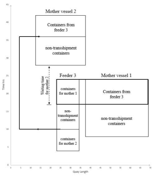
Figure 14. graphical representation of the solution

The model has run for about 8 secs to find the global optimal solution. Two different methods were used to verify the model results. An excel sheet with all necessary equations were created as first method of analysis. The output results from the model were used as input data to the excel sheet. The value of total cost resulting from the mathematical model was identical to the one from the excel sheet. A graphical representation of the results was generated to gain an insight about the earlier mentioned elements. As seen in Figure 14, there is no berthing location nor berthing time conflicts among vessels. In addition, containers transshipped directly from feeder #3 to mother vessel #1 has the same start and finish time for handling. Regarding indirect transshipment containers from feeder #3 to mother vessel #2, they start the handling after the unloading time from the feeder vessel. Lastly, the model was verified to have solution exactly as intended with no conflicts.

2          Chapter 4. Results and Discussion

This chapter describes how the proposed mathematical model, outlined in Chapter 3, can be used to handle the direct transshipment operations, and it also analyzes the corresponding computational results.

2.1         Transshipment hub layout

Very few studies address the direct transshipment method at container terminals as mentioned before. Some of those studies presented real data regarding the terminal configurations and costs of handling equipment based on surveys in different container terminals.  Some of the data developed by Zeng et al. (2017) was used in this study to generate test instances that illustrate the performance of the proposed approach. The model represents a terminal with 1380 meters continuous berth. Yard vehicles travel a distance of fifteen meters between quayside and yard side area (see Figure 15). It has twenty-four yard-blocks in total and each block is

100×15meters (

length×width) with the following margins:

• 15 meters between yard blocks horizontally
• 5 meters for handling lane at each yard block
• 10 meters as passing lane for trucks

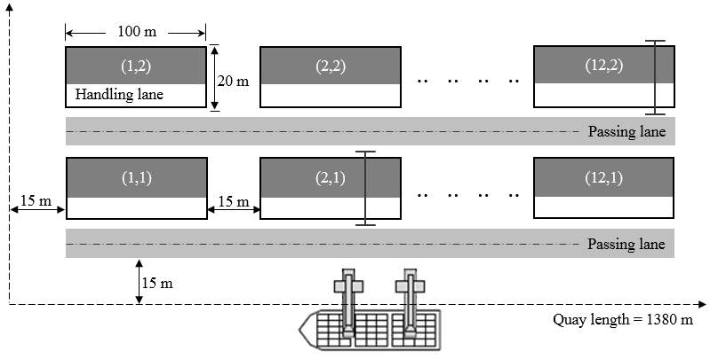
Figure 15. Schematic view of the terminal

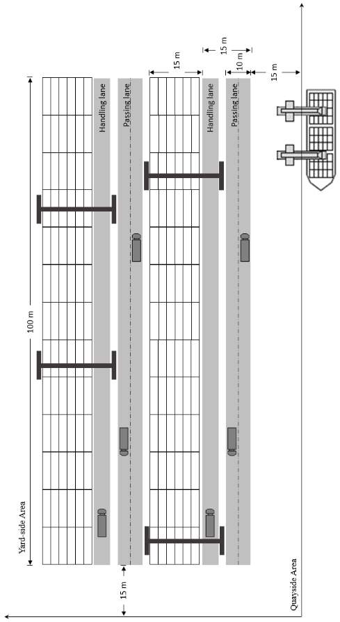
The length of each yard block is 16 containers TEU, the width is 6 TEUs and containers can be stacked up to 5 tiers. Hence, the capacity of each yard block is

16×6×5=480containers (TEU), with approximately 100 meters length (

16×6.06) and 15 meters width (

6×2.44). Note that the 20ft container dimensions are illustrated at Table 1. Figure 16 shows the detailed dimensions of the terminal yard blocks and indicates two yard-cranes deployed to handle containers at each yard block.

Figure 16. Yard block configuration

2.2         Scenario generation and input data settings

Table 6 lists cost parameters used in each scenario. There are penalty costs of mother and feeder vessels that the terminal must pay due to any delays in vessels’ expected departure times, in addition to the transportation and handling costs of yard trailers and cranes.

Table 6: Cost parameters used in each scenario

Item	Cost (USD)
Transport cost of yard trailers	0.0048 /m*TEU
Handling cost of yard cranes	4 /TEU
Penalty cost of mother vessels	160 /h
Penalty cost of feeder vessels	160 /h

The generated set has 2 mother vessels, 5 feeder vessels and 8 transshipment flows. Length of mother vessels is uniformly distributed between [250,390] meters, while feeders are within [80,120] meters. Arrival times of vessels are distributed along the planning horizon. Transshipment containers flow from feeder vessel to mother vessel with a uniformly distributed capacity between [100,400] TEUs. The study by Lee et al. (2013) stated some limitations on the transshipment relationship between mother and feeder vessels. By following those restrictions, mother vessels can have up to five flows coming from feeder vessels. On the other hand, feeder vessels can have transshipment relationships with up to two mother vessels at the same planning period.

The number of loading/unloading containers for mother vessels is ranging between [250,480] TEUs, however, containers for feeder vessels are within [150,400] TEUs. Unloading/loading containers and indirect transshipment containers are stored within defined yard sections. It is worthwhile to note that handling times for containers are calculated based on the assumption that there is one quay crane working to finish the handling operations for each vessel. The working speed of a quay crane is 40 TEU per hour as defined in Liang et al. (2012). Thus, the handling time for a vessel that has 360 TEUs is 9 hours. More accurate handling times for vessels can be defined by imposing the quay crane assignment problem within the proposed model constraints and decision variables.

Ten different scenarios are generated by randomly changing the input data (i.e., length of vessels, number of containers, and arrival time of vessels) within the previously mentioned distributions. (Omnia, make a table and show the parameter values for the ten scenarios) In addition, each scenario has different transshipment flows since the relationships between mother vessels and feeders are randomly determined. The assignment of containers to yard blocks also varies from one scenario to the other. Details of each scenario can be found in Appendix B.

2.3         Computational Results of the proposed model

The instances of the MILP model were solved by using Lingo 17.0 on an Intel i5 machine with 2.6 GHz CPU and 8 GB RAM with three hours computational time limit. Table 7 summarizes the results of the 10 scenarios. In Table 8, the number of direct transshipment flows as well as direct transshipment ratio resulted from each scenario are listed, while the total cost and direct transshipment ratio are depicted in Figure 17.

Table 7. Computational results of DTBAP model

Scenarios	Total cost	Time (min)	Delay cost		Operation cost
			Feeder	Mother	Transshipment containers	Loading/unloading containers
1	11,092.44	180	2240	160	5949.75	2742.68
2	8889.870	180	1280	160	6339.07	1110.80
3	11854.88	180	4000	160	5898.33	1796.55
4	10609.67	180	1920	0	6226.92	2462.75
5	10707.69	180	1440	0	6318.38	2949.32
6	12581.40	180	960	480	7790.44	3350.95
7	8067.072	180	800	320	4656.32	2290.76
8	15401.70	180	5440	1280	5582.19	3099.51
9	13830.55	180	3200	160	5436.45	5034.10
10	8283.715	180	1600	480	4585.5296	1618.19

Table 8. Direct transshipment ratio

Scenarios	Number of direct transshipment flows (a)	Direct transshipment ratio (a / 8) * 100
1	5	62.5%
2	4	50%
3	5	62.5%
4	5	62.5%
5	5	62.5%
6	5	62.5%
7	6	75%
8	6	75%
9	6	75%
10	7	87.5%

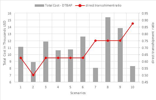
Figure 17. Total cost and direct transshipment ratio

Table 9 shows the recommended transshipment plan of containers for Scenario #7, where “zero” represents containers that will be transshipped directly between vessels, and “1” represents the traditional method being used for these containers. That is, transshipment containers between feeder #3 and mother vessel #1 are transported directly, for example. The result tables for other scenarios can be found in Appendix C.

Table 9. Recommended transshipment plan for Scenario #7

Feeder Vessel	3	4	5	6	7
1	0	1	0	–	0
2	0	1	–	0	0

The detailed berthing plan for Scenario #7 is depicted in Figure 18, where elements of vessels are illustrated in detail to better understand the schedule and sequence of the handling operations. Mother vessel #1 arrives to the terminal on the scheduled time and occupies its planned berthing position (b410). Mother vessel #1 starts the handling operation by loading containers directly from feeder #5. In such situation, mother vessel #1 becomes idle for about one hour waiting for the arrival of feeder #5. Once the feeder is allocated to berth segment b329, the unloading process of transshipment containers for mother vessel #1 starts immediately. Yard trucks transfer these containers along the berth and move a distance of 81 meters (

410-329) between feeder #5 and mother vessel #1. It is important to note that the start time of handling process for containers transshipped directly is set equal at both feeders and mother vessels. Non-transshipment containers of feeder #5 are handled immediately after finishing the unloading/loading process of transshipment containers for mother vessel #1.

Figure 18. Berthing plan for Scenario #7 Legend:
	Transshipment containers from feeder (5) to mother vessel (1)
	Non-transshipment containers for all vessels
	Transshipment containers from feeder (3) to mother vessel (1)
	Transshipment containers from feeder (7) to mother vessel (1)
	Transshipment containers from feeder (4) to mother vessel (1)
	Transshipment containers from feeder (6) to mother vessel (2)
	waiting time
	Transshipment containers from feeder (3) to mother vessel (2)
	Transshipment containers from feeder (7) to mother vessel (2)
	Transshipment containers from feeder (4) to mother vessel (2)

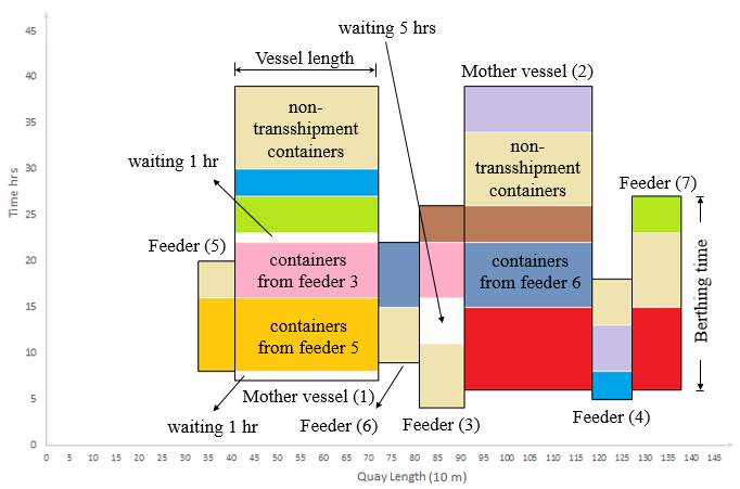
Feeder #3 non-transshipment containers are sequenced as the first job and handled as soon as the feeder arrives to the terminal and assigned to berth segment b810. There exist 5 hours waiting time for feeder #3 between the first and second sequenced handling jobs. This waiting time occurs not only because of using the direct transshipment method to transfer containers between feeder #3 and mother vessel #1, but also because of the assumption that handling operations cannot overlap and processed at the same time. Thus, feeder #3 waits for mother vessel #1 to finish handling containers coming from feeder #5. Mother vessel #1 becomes idle once again for one hour, while waiting for feeder #7 to finish handling all of its non-transshipment containers.

As indicated in Table 9, all transshipment containers are handled by using the direct method except for feeder #4. It is obvious from Figure 18 that feeder #4 does not have a direct relationships with mother vessels. Handling operations for feeder #4 are sequenced as follows: transshipment containers for mother vessel #1, transshipment containers for mother vessel #2, and finally handling the non-transshipment containers. Transshipment containers is exchanged between feeder # 4 and mother vessels #1 and #2 through the yard block area. Yard trucks transfer containers from berth segment 1185 to yard block (9,1) for the case of mother vessel #1 containers, and to yard block (3,1) for mother vessel #2 containers. Then, these containers are transferred again from the assigned yard blocks to the berthing positions of mother vessels. It is important to notice that, in the traditional method case, the start time of handling transshipment containers on mother vessels has to occur after the finish time of handling on feeder vessels.

2.4         Comparison with other planning model

The performance of the proposed model (let’s say DTBAP, which stands for direct transshipment berth allocation problem) is compared to the one from conventional berth allocation problem (BAP) model. Note that the BAP focuses only on the berth allocation of incoming feeders and mother vessels without considering the direct transshipment method. We formulated the BAP model similarly to the aforementioned one excluding the parameters and constraints related to the direct transshipment problem. The BAP model was also run for the same ten scenarios generated for DTBAP model and the corresponding solutions are reported in Table 10.

Table 10. Computational results of BAP model

Scenario	Total cost	Time (min)	Delay cost		Operation cost
			Feeder	Mother	Transshipment containers	Loading/unloading containers
1	13653.85	180	0	0	11885.35	1768.50
2	12965.57	180	0	0	11927.78	1037.79
3	13855.14	180	0	0	12704.46	1150.68
4	17220.59	180	0	0	14769.88	2450.72
5	14370.36	180	0	0	12043.86	2326.50
6	16086.01	180	0	0	13003.29	3082.72
7	13950.32	180	0	0	12281.72	1668.60
8	18250.85	180	0	0	15050.24	3200.61
9	18541.69	180	0	0	13993.78	4547.91
10	13764.85	180	0	0	10769.31	2995.54

Table 11 and Figure 19 compare the total cost of the two models for each of the ten scenarios. As can be seen, the total cost required for DTBAP model are significantly less than the one from BAP model for all of the ten scenarios. It is clearly seen that, by integrating the direct transshipment method along with the berth allocation problem, the total cost can be saved by 14% (Scenario #3) to 42% (Scenario #7).

Table 11. Comparison of total cost (DTBAP vs BAP)

Scenarios	Total Cost		% Reduction
	DTBAP	BAP
1	11,092.44	13653.85	19%
2	8889.870	12965.57	31%
3	11854.88	13855.14	14%
4	10609.67	17220.59	38%
5	10707.69	14370.36	25%
6	12581.40	16086.01	22%
7	8067.072	13950.32	42%
8	15401.70	18250.85	16%
9	13830.55	18541.69	25%
10	8283.715	13764.85	40%

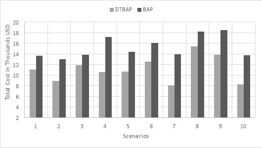
Figure 19. Comparison of total cost (DTBAP vs BAP)

As can be seen in Figure 20, penalty cost of vessels is negligible in BAP model. It is obvious that feeder vessels delay cost is much higher than the penalty cost for mother vessels, on average. This is due to the assumption that feeders arrive at the terminal before mother vessels. From the economic perspective, it is not desirable for mother vessels to wait longer than the scheduled time at terminals, since they travel long distances carrying large number of containers. Based on this fact, feeders’ arrival time assumption is used to generate input data that impacts the vessels’ penalty cost.

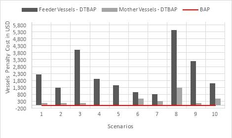
Figure 20. Penalty cost comparison

DTBAP model also requires less operational cost for transshipment containers than the BAP model as shown in Figure 21. Because of the closeness of feeders and mother vessels arrival times, it is more economically for terminal management to pay penalty costs for shipping liners than transporting containers back and forth between quayside and yard side area within such a short time period. As a result, we may conclude that considering the direct transshipment method will lead to a significant amount of cost savings while operating container terminals.

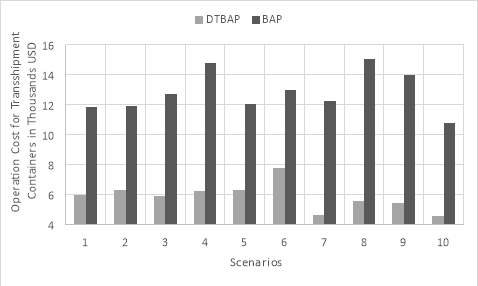
Figure 21. Transshipment containers operational cost

2.5         Sensitivity Analysis

The model decides either to use the direct transshipment method or not based on a comparison between two cost parameters. When containers are transshipped through the terminal yard blocks, gantry crane cost besides truck transport cost are important input parameters that determine the total cost. Meanwhile, penalty cost of vessels in addition to yard trucks cost, is the key factor that influences total cost while implementing the direct transshipment method. Delay cost of vessels is pre-determined by and highly dependent on shipping liners. However, transportation and handling costs of yard trucks and gantry cranes are assigned by terminal operators and mainly based on the handling equipment used at the port. Consequently, the performance of DTBAP and BAP models are analyzed and compared with different values of these input parameters.

2.5.1        Transport cost

The increase in yard trucks transport cost, the total cost of the two models increases accordingly. This is due to the involvement of yard trucks to transport containers regardless of the assigned transshipment method. It is obvious that indirect transshipment containers travel much longer distances which result in higher objective function value for BAP model.

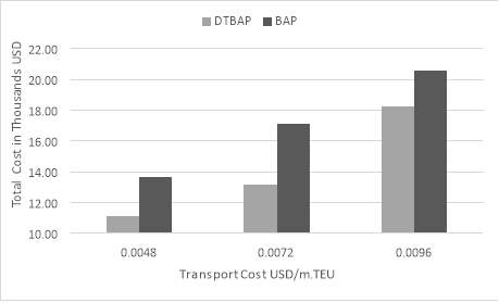
Figure 22. Transport cost of yard trucks for scenario (1)

2.5.2        Feeder vessel delay cost

As can be seen in Figure 23, the increase of feeder vessels penalty cost has no significant effect on the total cost of BAP model, however, the total cost for DTBAP increases gradually. In addition, the direct transshipment ratio which is calculated by (number of container groups handled directly/the total number of transshipment flows) decreases when the penalty cost increases. For Scenario #7 there were 6 transshipment flows out of 8 is handled directly when feeder penalty cost is set to 160 USD/hr. However, this ratio dropped down to 5 transshipment flows when the penalty cost is set to either 200 or 240 USD/hr. Thus, when the penalty cost increases, terminal operators might pay less cost by indirectly transshipping containers.

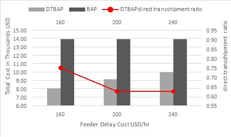
Figure 23. delay cost of feeders for scenario (7)

2.5.3        Gantry crane cost

As indicated in Figure 24, by increasing the gantry crane cost, the total cost of the two models increases. It is important to mention that the BAP model total cost increases with a higher rate than the DTBAP model. This is due to the fact that all the transshipment flows are handled indirectly at the BAP model. The lower increase rate at the DTBAP model can be explained since only few transshipment flows are handled through the terminal yard area. Furthermore, the DTBAP model tends to have higher direct transshipment ratio with increases in gantry crane cost.

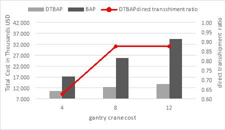
Figure 24. gantry crane cost USD/TEU

2.5.4        Arrival Time of Vessels

It is worthwhile to note that the direct transshipment decision depends mostly on the gap between the arrival times of feeders and mother vessels. As the gap increases, feeder vessels tend to wait idle for longer times which cause terminal management to pay more penalty cost. Based on the economical comparison achieved by the proposed mathematical model, it might be a better solution to transship those containers using the traditional method. Therefore, it is very important to analyze the model results alongside with the direct transshipment ratio while changing vessels arrival times. Since the transshipment ratio is more than 50% as given in Table 8. Another 10 scenarios were generated with the same input parameters except for feeders’ arrival times schedule. It moves a bit forward so all arrival times are 2 hours earlier than the original schedule.