Applications of Monte Carlo Methods

Monte Carlo General

From the early 1900’s many scientists were trying to find solutions to difficult and extensive problems. But all faced the same problem, the countless calculations. In the 1930’s, Enrico Fermi first experimented with the Monte Carlo method while studying neutron diffusion, but he did not publish anything on it. Before the first computer, calculations were being done by hand. Many universities were using their students, and mostly the females, for that tough job. Thus, from the beginning there was the need of a machine to make fast and accurate calculations. During 1940 many scientists were working on nuclear physics, and more specifically to nuclear bombs. Then the biggest problem was neutron diffusion. Apparently, the difficulties were great. First, there wasn’t any way to know exactly what a neutron diffusion will cause, except if that became by experiment. Of course, that was dangerous in terms of radiation and power to the staff. Therefore, there was the need of stimulation. By stimulate a neutron diffusion, the ‘’experiment’’ would be really helpful and bring many information but most important it would be safe. Fortunately, the scientist Von Neumann came to find the solution. Von was working at the University of ? . One day he was ill he was playing cards and he thought how is it possible to win every single game? The answer was simple, if someone play many many games and create a pattern then he will know that every movement will have a possibility to ‘’drive’’ him to a win. But the problem was that number of plays. Thusly, after discussing his idea with 2 other scientists and following by the first computer creation ENIAC they build a program that would be able to make this calculation faster and more accurately from humans. The name had been given by ? , Monte Carlo. The name came from an uncle of ? who were taking money from relatives for gambling in Monte Carlo Casino. Statistical sampling was known in mathematics before, but now they had the opportunity to make the calculation and take the results fast. Their weapon was the creation of random numbers, which lead them to have different ‘’experiments’’ simultaneously. But to be more precisely pseudo-random numbers, because a computer can’t give random numbers. Finally, computer and Monte Carlo were able to give simulations for many occasions. The first use was about neutron diffusion. Now the had a safe and fast way to see the neutron diffusion without any damage. The roots were existed. From physics, they knew the laws that neutrons follow, the geometry of the machines. So, everything was ready for the imaginary experiment. The problem was that that experiment would help for the development of a nuclear bomb. Fortunately, the experiment worked but never used for the creation of a massive destruction weapon. That’s the beginning of the new era which gave to everyone a tool to make simulations of what they need. Before the Monte Carlo method was developed, simulations tested a previously understood deterministic problem, and statistical sampling was used to estimate uncertainties in the simulations. Monte Carlo simulations invert this approach, solving deterministic problems using a probabilistic analog.

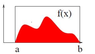
Monte Carlo methods are a broad class of computational algorithms that rely on repeated random sampling to obtain numerical results. Their essential idea is using randomness to solve problems that might be deterministic in principle. They are often used in physical and mathematical problems and are most useful when it is difficult or impossible to use other approaches. Monte Carlo methods are mainly used in three problem classes:optimization, numerical integration, and generating draws from a probability distribution

General idea is “Instead of performing long complex calculations, perform large number of experiments using random number generation and see what happens”. Monte Carlo assumes the system is described by probability density functions (PDF) which can be modeled. It does not need to write down and solve equation analytically or numerically.

In physics-related problems, Monte Carlo methods are useful for simulating systems with many coupled degrees of freedom, such as fluids, disordered materials, strongly coupled solids, and cellular structures.

Monte Carlo methods find application in a wide field of areas, including many subfields of physics, like statistical physics or high energy physics, and ranging to areas like biology or analysis of financial markets. Very often the basic problem is to estimate a multi-dimensional integral.

In principle, Monte Carlo methods can be used to solve any problem having a probabilistic interpretation. By the law of large numbers [Law of large numbers (LLN) is a theorem that describes the result of performing the same experiment a large number of times. According to the law, the average of the results obtained from a large number of trials should be close to the expected value, and will tend to become closer as more trials are performed], integrals described by the expected value of some random variable can be approximated by taking the empirical mean (a.k.a. the sample mean) of independent samples of the variable. When the probability distribution of the variable is parametrized, mathematicians often use a Markov chain Monte Carlo (MCMC) sampler. The central idea is to design a judicious Markov chain model with a prescribed stationary probability distribution. That is, in the limit, the samples being generated by the MCMC method will be samples from the desired (target) distribution. In other problems, the objective is generating draws from a sequence of probability distributions satisfying a non-linear evolution equation. These flows of probability distributions can always be interpreted as the distributions of the random states of a Markov process whose transition probabilities depend on the distributions of the current random states. In other instances, we are given a flow of probability distributions with an increasing level of sampling complexity (path spaces models with an increasing time horizon, Boltzmann-Gibbs measures associated with decreasing temperature parameters, and many others). These models can also be seen as the evolution of the law of the random states of a nonlinear Markov chain. A natural way to simulate these sophisticated nonlinear Markov processes is to sample a large number of copies of the process, replacing in the evolution equation the unknown distributions of the random states by the sampled empirical measures. In contrast with traditional Monte Carlo and MCMC methodologies these mean field particle techniques rely on sequential interacting samples. The terminology mean field reflects the fact that each of the samples (a.k.a. particles, individuals, walkers, agents, creatures, or phenotypes) interacts with the empirical measures of the process. When the size of the system tends to infinity, these random empirical measures converge to the deterministic distribution of the random states of the nonlinear Markov chain, so that the statistical interaction between particles vanishes.

For 1-dimension integral I=

∫dxf(x)

This can be approximated by pulling N random numbers xi, i = 1 . . .N, from a distribution which is constant in the interval a ≤ x ≤ b:

The solution of that integral is I ≈

b-aN ∑i=1Nf(xi).The result becomes exact when N → ∞. Consequently, by considering n dimensions: I=

∫Vdnx f(x). For simplicity, V is the volume of a n-dimensions hypercube, with 0 ≤ xμ ≤ 1. That Monte Carlo integration generates N random vectors xi from flat distribution

(0 ≤ (xi)μ ≤ 1). As N → ∞,

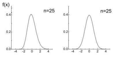
the solution tend to, I→VN∑i=1Nf(xi).The error ∝ 1/√N and independent of the dimensions n. This is due to the central limit theorem.

In Monte Carlo the most efficient algorithm depends on a specific problem. The more are known about the specific problem, the higher the chances to find an algorithm which solves the problem efficiently. Monte Carlo integration offers a tool for numerical evaluation of integrals in high dimensions. Furthermore, Monte Carlo integration works for smooth integrands as well as for integrands with discontinuities. This allows an easy application to problems with complicated integration boundaries.

However, the error estimate scales always with 1/√N. To improve the situation, we introduced the classical variance reducing techniques.

Monte Carlo depends on random numbers. Since a computer is a deterministic machine, truly random numbers do not exist on a computer. Thusly the solution is to use pseudo-random numbers. Pseudo-random numbers are produced in the computer deterministically by a simple algorithm, so they are not truly random, but any sequence of pseudo-random numbers is supposed to appear random to someone who doesn’t know the algorithm. More quantitatively one performs for each proposed pseudo-random number generator a series of tests T1, T2, …, Tn. If the outcome of one test differs significantly from what one would expect from a truly random sequence, the pseudo-random number generator is classified as “bad”. Note that if a pseudo-random number generator has passed n tests, we cannot conclude that it will also pass test Tn+1.

In this context also, the term “quasi-random numbers” appears. Quasi-random numbers are not

random at all but produced by a numerical algorithm and designed to be distributed as uniformly as possible, to reduce the errors in Monte Carlo integration.

Consequently, a good random pseudo-number generator should satisfy some criteria.:

• Good distribution. The points should be distributed according to what one would expect from a truly random distribution. Furthermore, a pseudo-random number generator should not introduce artificial correlations between successively generated points.

• Long period. Both pseudo-random and quasi-random generators always have a period, after which they begin to generate the same sequence of numbers over again. To avoid undesired correlations, one should in any practical calculation not come anywhere near exhausting the period.

• Repeatability. For testing and development, it may be necessary to repeat a calculation with the same random numbers as in the previous run. Furthermore, the generator should allow the possibility to repeat a part of a job without doing the whole thing. This requires to be able to store the state of a generator.

• Long disjoint subsequences. For large problems it is extremely convenient to be able to perform independent sub simulations whose results can later be combined assuming statistical independence.

• Portability. This means not only that the code should be portable (i.e. in a high-level

language like Fortran or C), but that it should generate exactly the same sequence of numbers on different machines.

• Efficiency. The generation of the pseudo-random numbers should not be too time-consuming.

Almost all generators can be implemented in a reasonably efficient way. To test the quality of a pseudo-random number generator it is necessary performing a series of test. The simplest of all is the frequency test. If the algorithm claims to generate pseudo-random numbers uniformly distributed in [0, 1], one divides this interval into b bins, generates n random number u1, u2, … un and counts the number a pseudo-random number falls into bin j (1 ≤ j ≤ b). One then calculates χ2 assuming that the numbers are truly random and obtains a probability that the specific generated distribution is compatible with a random distribution. The serial test is a generalization of the frequency test. Here one looks at pairs of successive generated numbers and checks if they are uniformly distributed in the area [0, 1] × [0, 1].

The ultimate goal for Monte Carlo simulation is to mimic the nature. Monte Carlo in physical science is a huge field of research: a major factor of the supercomputing resources in the world is used in physical simulations. There are 2 methods to obtain predictions from a given physical theory, analytical estimations and computer simulations. Analytical estimations cannot be used for long and complicated problems as for example lepton and hardon physics because these physical systems many behaviors. However, in practice these always rely on either simplifying assumptions or some kinds of series expansions (for example, weak coupling): thus, both the validity and practical accuracy are limited. In several fields of physics research computer simulations form the best method available for obtaining quantitative results. With the increase of computing power and development of new algorithms new domains of research are constantly opening to simulations, and simulations are often necessary in order to obtain realistic results.

Computing simulation give the probability that a process happens with given kinematics and simulate kinematics of event according to cross section. Besides it needs a mechanism to select a given configuration according to a probability density function by using of Random Numbers and Monte Carlo Method. Monte Carlo method refers to any procedure that makes use of random numbers

uses probability statistics to solve the problem. Monte Carlo methods are used in Simulation of natural phenomena, Simulation of experimental apparatus. Monte Carlo use Pseudo Random Numbers, which are a sequence of numbers generated by a computer algorithm, usually uniform in the range [0,1] more precisely: algo’s generate integers between 0 and M, and then

rn=

InM.Besides Monte Carlo follows the Law of large numbers. It chose N numbers

uirandomly, with probability density uniform in [a,b], evaluate f(ui) for each ui , for large enough N Monte Carlo estimate of integral converges to correct answer. Central Limit Theorem for large N the sum of independent random variables is always normally (Gaussian) distributed

For these reasons CERN uses Monte Carlo techniques in all the experiments which occurred all these forming years. CERN is a national institute which has as a goal to unlock the mystery of particle physics, during researching in many different aspects of science. Particle physics follow the law of quantum mechanics. Thus, is impossible to know the results from the beginning of an experiment. But thankfully the law and the contribution for each reaction is known. Consequently, Monte Carlo is the most powerful tool in CERN. In CERN the Monte Carlo generators are combined with detector simulations (Geant). This is used for accelerators and collisions and it’s an event generator. Besides it’s used for detectors and electronics for detector simulations. The main procedure for an experiment is the following

Choose model, constraints, parameters, decay chain of interest -> Kinematics, information from a known (detectable) particles->Detector Simulation (Hardware, Software)->Offline software (Event selection)->Results Improvement

The role that Monte Carlo methods play in the physical sciences & Radiotherapy

Over the last four decades, numerical computation has played an increasingly vital role in both theoretical and experimental science. The rising sophistication of our understanding of physical phenomena coupled with our growing need to create even more subtle processes and devices involves a level of analysis and prediction beyond that of traditional mathematical methods. For example, is someone wants to design a modern high-energy accelerator, any of its enormous detectors, a proposed experiment, or to analyze the results, computation has to be invoked at every stage of the procedure. Inference from most astronomical observations is usually a matter of significant computer-aided analysis. An opposite situation exists in theoretical science. Serious quantitative prediction of a chemical reaction rate, the behavior of a nuclear reactor, or the energy of an atomic nucleus from more fundamental information demands computation, often very demanding. Monte Carlo methods play a fundamental role in many of these computations. For example, the prediction of behavior of a high-energy particle detector is most straightforwardly and most precisely analyzed by a Monte Carlo method that simulates the stochastic procedures of the formation of particles in a target, the decay of those particles into others, the transport of particles, and their final interactions with the detection process. Such a calculation is formidable but straightforward on present computers. Because the computation deals with a series of independent histories, it is easily parallelized too. It is also worth declaring that the full explanation of the state of a particle decay process in a particle detector needs many dimensions, there may be a number of particles instantaneously present in the system, and for each a position, time, and momentum must be quantified, a total of seven dimensions for each particle. Monte Carlo methods recommend a natural and proficient procedure for numerical problems in many dimensions that are impossible by more traditional numerical methods. Monte Carlo algorithms use a computer program, a process or a subroutine, called “random number generator” (RNG). On the other hand, computers cannot really create “random” numbers because the output of any program is, by definition, predictable. Consequently, it is not truly “random.” Hence, the result of these generators shall correctly be called “pseudorandom numbers”. A huge sequence of these pseudorandom numbers is obligated to solve a dense problem. The numbers within an order of random numbers shall be uncorrelated, that is, they must not depend on each other. Because this is impossible with a computer program, they should at least look like independent. In other words, any statistical test program shall confirm that the numbers within the sequence are uncorrelated and any computer code that involves independent random numbers shall produce a similar result with different sequences. If this is the case within the uncertainty of the simulation, then these sequences can be called pseudorandom. A pseudo-RNG must be examined sensibly before it can be used for a specific purpose. A beneficial generator for simulations in radiation therapy must offer two important features: 1) The period of the sequence shall be large enough. Otherwise, if the sequence is reused several times, the results of the MC simulation are correlated. 2) They must be consistently distributed in multiple dimensions. That means random vectors created from an n-tuple of random numbers must be consistently distributed in the n-dimensional space. Normally, it is not obvious how to spot correlations in higher dimensions. Most of the generators deliver uniformly distributed random numbers in some interval, typically in [0,1]. One class of simple RNGs is called linear congruential generators. They generate a sequence of integers I₁, I₂, I₃, . . ., each between 0 and m − 1 by the recurrence relation:

I_j+1=aI_j+c with the parameters

a: multiplier

c: increment

m: modulus

Basics of Measurement Dosimetry of Photon and Electron Beams Theory of Measurement Dosimetry

 

The determination of absorbed dose is presented using a radiation detector in a reference dosimetry setup, expressed by the radiation source and geometry of interest. By achieving an experimental measurement of the detector reading or signal in these conditions, one can gain the absorbed dose to the medium of interest by altering the detector signal, being stimulated by a physical process precise to the device, to absorbed dose to the medium at the point of measurement. The suitable corrections have been operated to the detector signal, (1) refer to usual reference conditions (e.g., environmental conditions in ionization chambers) and (2) correct for effects that change the measurement of the physical process itself (e.g., ionization chamber recombination and polarity effects). The result is called detector signal. Note that Monte Carlo calculations can also play a role in the purpose of these corrections. The detector signal is first transformed to absorbed dose in the sensitive volume of the detector, also called the detector cavity. For a certain detector signal M_det, the absorbed dose in the detector cavity, denoted D_det, can be expressed as D_det = C_QM_det, where C_Q is a international factor representing the switch of detector signal to absorbed dose in the detector cavity for a specific beam quality Q. The factor depends on the physical detection mechanism and incorporates the inherent energy dependence of the detector, its linearity with dose and its dose rate dependence. Note that C_Q can also be stated as the product of a series of factors, each accounting for these effects. The essential energy dependence describes the relationship between the physical effect and the dose to the detector sensitive volume. In practice, the intrinsic energy dependence is typically established indirectly, by calibration against a standard at a specific beam quality (e.g., 60Co for linac radiotherapy) and after obtaining the extrinsic energy dependence as calculated by condensed history (CH) Monte Carlo methods. The importance of differentiating intrinsic and extrinsic energy dependence lies in the aptitude to verify the impact of beam quality change on the response of a detector arising from fundamental effects versus dosimetric effects that can be exhibited through CH Monte Carlo techniques. Absorbed dose in the detection cavity to absorbed dose to medium, considering the detector in its entire physical integrity, is written as, D_med =f D_det, where D_med is the absorbed dose to the medium at the point of measurement and f is a factor demonstrating the overall absorbed-dose energy dependence of the detector. During radiation transportation, the density of ionizations in charged particle tracks is much greater than for photons, which in rule interact only once, and as a result the contribution of charged particles to dose is prevailing, whether the primary beam is a photon or electron beam. Moreover, as electrons are set in motion by ionization, their fluence is higher than for positrons, characteristically by at least a few orders of magnitude for radiotherapy beams. Then, collision mass stopping power be close to over the electron spectrum is a major indicator of the absorbed-dose energy dependence of the detection material, with regard to the overall solution of Boltzmann radiation transport equations achieved by the Monte Carlo method. This means that even for an markedly small detection cavity, unfettered of the effect of components, the adaptation of absorbed dose to the detector to absorbed dose to medium must reflect the energy dependence of the mean mass stopping power, which is expressed by the electron fluence spectrum and the physical assets of the media. The detector can be expressed as the ratio of its reading, M_det, to the quantity of interest, which could be air kerma or dose to a medium. For example, the detector absorbed dose response or sensitivity is defined as R_D =

MdetDmed, where M_det is the reading of the detector placed in the medium and D_med the absorbed dose at the effective point of measurement in the medium.  The absorbed dose response can be written as R_D =

1fCQ. Monte Carlo simulations of detector response are involved with the extrinsic component of the response, that is, the calculation of f.

In-Phantom Dosimetry

 

Absorbed dose measurement techniques are precise to a given detector, geometry, and beam quality. In radiation dosimetry, the beam quality should be regarded as a beam-specific and geometry-dependent concept, rather than an expressive of the beam only. It is outlined as the overall situation induced by a given radiation beam in a specific region of the geometry of interest. While this condition is multidimensional, quality can be related to dosimetric factors being detector specific and Monte Carlo Techniques in Radiation Therapy position dependent. Practically, beam quality is encapsulated in a single quantity known as the in-water beam quality specifier. This quantity is used in particular applications where dosimetric factors need to be characterized as a function of beam quality. The function C_Q and the factor f, correspondingly, depend on the nature of the detector and the beam quality. For a given beam quality, the standard formalism to convert detection signal to absorbed dose in the detection cavity is CQ Ngas , where Ngas is a signal-to-dose calibration coefficient that can be expressed as (4.6) Here, (W/e)gas is the energy necessary to create an ion pair in the gas filling the chamber for a cobalt-60 beam (e.g., 33.97 eV/ pair for sea-level dry air (Boutillon and Perroche-Roux, 1987)) and mgas is the mass of gas (air) in the effective sensitive volume of the chamber. The absorbed-dose energy dependence factor f, used to convert detector dose to dose to medium, is expressed as where (L/ )gas ρmed is the medium-to-gas Spencer–Attix stopping power ratio, representing the absorbed-dose energy dependence of the detection material, Prepl is the replacement perturbation factor, and Pwall, Pcel, and Pstem are the wall, central electrode, and stem perturbation factors, respectively. where Pi are the component-specific perturbation factors of the detector.

Air Kerma Dosimetry

Air kerma measurements with ionization chambers have been,for several decades, fundamental to clinical radiation dosimetry. In practice, a thick wall of air-equivalent material is chosen to enclose the air cavity, such that the perturbation of the electron spectrum between the wall and the air is minimal. The beam quality-specific wall thickness is chosen larger than the electron range (in the wall material), such that electron equilibrium(strictly speaking, a transient equilibrium) is established between the photon beam and secondary electrons in the wall. The rationale is to convert absorbed dose in the detection cavity filled with wall material into absorbed dose to the medium consisting the geometry. Assuming that th eattenuation of the photon fluence in the wall and the medium are identical, this is achieved by simply taking the ratio of collision kerma wall-to-medium, as follows:Kcoll,med  (4.10)

where (μen ρ)wall med / is the ratio of mass–energy absorption coefficients, medium-to-wall. In Equation 4.10, it is implicitly assumed that the photon energy fluence in medium (air) and wall is identical, and that there is perfect CPE in the wall (i.e., Kcoll,wall = Dwall).

.

Interaction Coefficients

 Other important quantities of interest that can be calculated with Monte Carlo simulations are mass–energy absorption coefficients. In the context of dosimeter response for in-air and in-phantom measurements, several studies have addressed kilovoltage photon beams   as well as high-energy photon beams. Calculated data have been used to obtain correction factors in respect to dosimetry . The average mass-absorption coefficients in a given medium is defined as follows:  (4.17) where φγ(hν) is the photon fluence differential in energy (in MeV−1 cm−2), μis the energy-dependent linear attenuation coefficient in the medium (in cm−1), and Eab(hν) is the average energy being absorbed by the medium from photon interactions with initial energy hν. Note that one needs Monte Carlo simulations to evaluate Eab(hν). The evaluation of such coefficients requires linear attenuation data and a proper knowledge of the photon fluence spectrum, either measured or calculated with Monte Carlo simulations under specific conditions. Systematic compilations of mass–energy absorption coefficients for elements and materials of dosimetric interest were performed by Hubbell (1982) and Seltzer (1993) for monoenergetic photons. To avoid storage of a large number of spectra, direct scoring techniques with Monte Carlo can be used to calculate average ratios under specific conditions

Modeling Detector Response

4.4.1 Ionization Chamber Correction Factors

Over the last decades, considerable improvements in particle transport accuracy   have allowed the use of Monte Carlo methods for detector response simulation to an accuracy of 0.1% or better. Such improvements have allowed studies to be performed in dosimetric situations that could not be done by other means with the same level of accuracy.  In general, detector sensitivity (or response) calculations cover three areas of importance: (1) in-phantom reference dosimetry, (2) in-phantom relative dosimetry, and (3) in-air chamber correction factors.

For relative dosimetry, Monte Carlo modeling of ionization chamber response has been applied to aid an accurate conversion of depth ionization into depth dose for both photon and electron beams. In electron beams, this entailed calculation of stopping-power ratios (Burns et al., 1995) and perturbation correction factors as a function of depth (Buckley and Rogers, 2006a,b; Verhaegen et al., 2006).

In photon beams, stopping-power ratios have been shown to be quasi-depth independent, except for the build-up region (Andreo and Brahme, 1986) but recent efforts have readdressed the issue of the EPOM in the determination of percent depth dose.  Other detectors have also been modeled in the context of relative dosimetry. Diode detectors are very efficient for electron beam PDD measurements, since at clinically relevant depths when placed with the center of the sensitive volume at the appropriate depth, measured reading does not require any correction. However, because electrons reach sub-MeV kinetic energy in the high-gradient region of the PDD curve beyond dmax and because the relative contribution of bremsstrahlung photons to dose increases for depths beyond dmax, one might expect that the response of the diode must be corrected in this dose fall-off region and especially the bremsstrahlung tail

 

Simulation Geometries

 

In general, common Monte Carlo systems provide a geometry package in which radiation transport is simulated. In the context of photon and electron beam radiation therapy, accurate detector response calculations are performed using mainly two systems: (1) EGSnrc (Kawrakow, 2000a) and (2) PENELOPE (Salvat et al., 2009). Both systems have powerful tools to describe detector geometries.  Typical userdefined geometry can be done using simple solids such as boxes, spheres, or cylinders along with the use of Boolean operators (union, intersection, etc.) on these objects to combine them logically and make complicated geometries. Also, geometries can be defined by the surfaces surrounding them.

General Considerations

In assessing the accuracy of Monte Carlo calculated detector response, there are four main sources of systematic uncertainties:

1. The accuracy of the CH transport system

2. The accuracy of the cross-section data in the system, including both fundamental properties of elements

(I-values, etc.) and how well the true composition of the materials of the real detector are modeled (impurities, etc.)

3. The accuracy of the geometry of the model of the detector

4. The accuracy of the radiation source model (i.e., small field, collimation system, spot size, etc.)

Monte Carlo Modeling of External Photon Beams in Radiotherapy

 

Intro

It is well acknowledged that Monte Carlo simulation methods proffer the most dominant tool for modeling and analyzing radiation transport for radiotherapy applications. One of the most common and crucial uses of Monte Carlo modeling in external beam radiotherapy is the establishment of a virtual model of the radiation source. Applications are source design and optimization, studying radiation detector response and treatment planning. Since the clear majority of radiotherapy is performed with megavolt (MV) photon beams from a linear accelerator (linac), this is also reflected in the research efforts. External beam radiotherapy is operated with electron beams, lower-energy photon beams emanating from an x-ray tube, or hadron beams. Nowadays, clinically operated photon beams in radiotherapy usually are within the energy range of 4–25 MeV. A linac has a basic modular construction as shown generically in Figure 1.

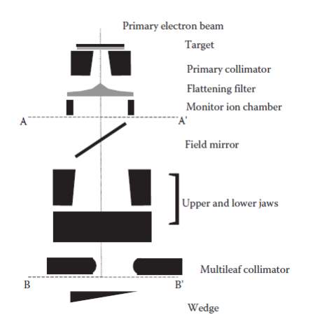
Components of a Monte Carlo Model of a Linac Photon Beam

 

The components illustrated in Figure1 must be known meticulously to build an accurate model of a linac. The composition of materials and compounds (their mass densities), the position, dimensions, and shape of defining surfaces of the components; and their motion must all be known in great specificity to build an accurate Monte Carlo model. Knowledge of acceptances may help to determine uncertainties in the calculated results. Errors made at this stage will often translate into systematic errors in the calculated output of the linac. Therefore, it is of utmost significance that linac blueprints are verified as much as possible and that Monte Carlo linac models are certified against an extensive set of dose measurements of depth and lateral dose profiles in water. The validation procedure may include evaluations against measurements at various source-to-surface distances of a phantom.

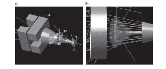Figure 2 shows a characteristic example of a simple photon linac model. The Figure 2a presents the linac components and particle tracks the figure 2b illustrates the interactions in the flattening filter. The BEAM code allows easy assembly of a linac model with a wide choice of building blocks consisting of geometrical shapes such as disks, cones, parallelepipeds, trapezoids, and so on. The code depends heavily on the fact that linac parts do not overlap in the beam direction, which is mostly the case. Separate parts of a linac are able to be built, validated, and studied separately. Furthermore, particle transport can be accomplished for electrons, photons, and positrons. Particles can be attached according to interaction types and interaction sites which offer a powerful beam analysis method.

The photon linac components that are the most valuable in the model in Figure 1 are the target, flattening filter, secondary collimators such as jaws and multileaf collimator (T, FF, SC), and wedges. After the accelerated primary electron beam departs the flight tube, it has a narrow-energy, angular and spatial distribution. This electron beam will attain the target, regularly consisting of a high-Z metal in which the electrons will generate bremsstrahlung photons. Target and flattening filters are the most significant sources of contaminant electrons, unless a wedge is attended. In the model of Figure 1, there are two more components, the monitor ion chamber and the field mirror. Both offer only a small attenuation to the photon beam and are often omitted from Monte Carlo models. Finally, the photon beam is formed and moderated by secondary collimators and beam modifiers such as jaws, blocks, multileaf collimators (MLC) and wedges.

Primary Electron Beam Distribution and Photon Target

 

Photon Target Simulation for Radiotherapy Treatment

 

The bremsstrahlung photons generated in the target by the primary electrons in the energy range 4–25 MeV are mostly originated from a fairly thin layer on the upstream side. This is because of the fast energy degradation of the electron energy in a high- Z material, the almost linear reliance on the bremsstrahlung cross section on the electron kinetic energy for high energies and electron scattering in the target. At high electron energies, the average bremsstrahlung photon emission angle is given approximately by m₀c²/E₀ (m₀c² is the electron’s rest energy and E₀ its total energy) producing a strongly forward-peaked angular distribution. Targets in clinical linacs are ordinarily thick enough to block the primary electrons completely and are for that reason often referred to as “thick targets.” In such targets, the bremsstrahlung photon angular distribution will be spread out because of electrons undertaking multiple scattering, but the result will on the other hand be a strongly anisotropic photon fluence, while the photon spectrum is moderately isotropic. More complex analytical calculation schemes have been acquired but the most widespread method to generate bremsstrahlung photon distributions from targets in clinical linacs is Monte Carlo simulation. It involved a 5.7 MeV electron pencil beam attaining a W/Cu target, followed by a flattening filter of Pb and an unspecified collimator. For several combinations of target materials and flattening filters, there is a linear correlation between the depth of the dose maximum in water and the average energy of the photon spectrum escaping the linac for 10–25 MV photon beams. Thus, Monte Carlo simulations are a overwhelming tool for designing target and flattening filter.

Photon Beam Spot Size in Radiotherapy Accelerators

 

A point that deserves special attention is the focal spot size of the photon beam or the primary electron beam. The focal spot size is a vital parameter in Monte Carlo simulations, which influences calculated dose and fluence distributions.

Flattening Filter

 

Flattening filter has a major influence on the beam. Flattening filters are originated to generate flat dose distributions at a certain depth in water. Monte Carlo simulations illustrate the influence of the usually complex-shaped flattening filter on photon fluence distributions. Flattening filters affect significant spectral hardening both on and off the beam axis. The bremsstrahlung spectrum from a thick target is fairly isotropic within the angular range of the photons that can reach the patient, whereas the bremsstrahlung intensity is highly anisotropic.

Monitor Ion Chamber Backscatter

In some clinical linacs, the signal from the beam monitor ion chamber is influenced by the spot of the secondary movable beam collimators (jaws). This only befalls in linacs where the distal monitor chamber window is adequately thin, where no backscatter plate is present and where the distance between chamber and the upper surface of the collimators is small enough. Therefore, particles backscattering from the movable collimators can deposit charge in the monitor chamber, as well as particles moving in the forward direction in the beam. In a small field, more backscatter from the collimators will take place than in a large field. This means that the monitor chamber will attain its preset number of monitor units (MU) rapider and terminate the beam. This will trigger the linac output to decrease with reducing field size. The magnitude of this effect is typically limited to a few percent but for some linac types, larger effects have been reported. The decreased output is automatically comprised in output factor measurements, but when Monte Carlo simulations are used to settle output factors, the effect has to be taken into account individually. This applies to all cases where outputs from fields of different sizes are combined. Monte Carlo techniques are used too, to examine the backscatter effect. By tagging particles and selectively transporting photons and electrons, it was found that electrons cause most of the backscatter effect. A spectral analysis of the forward and backward moving particles was shown.

Wedges

Including a physical wedge in a photon beam modifies the beam characteristics significantly. Not only is the dose distribution changed by attenuation and scatter from the wedge, but also the photon spectrum is also influenced. Besides, when a moving linac jaw is used to shape a dynamic (or virtual) wedge, the photon spectrum is much more alike to the open-field spectrum. For very-high energy beams (>20 MV), beam wedges may cause beam softening due to, for example, pair production and annihilation. Monte Carlo simulations can be operated to model physical or dynamic wedges. When modeling a physical wedge, great care must be taken that the model for the wedge is precise. Not only the exact shape of the wedge has to be implemented, but the composition and density also have to be known precisely. In forming Monte Carlo models for dynamic wedges, the time-dependent movement of the jaw has to be included.

Full Linac Modeling

The photon beam models can be principally divided into two categories. The first approach is to execute complete simulations of linacs and either custom the obtained particles straight in calculations of dose and fluence in phantoms or store phase-space data about these particles at possibly several planar levels in the linac for further use. The phase-space can be experimented for further particle transport in the rest of the geometry (linac or phantom). If the phase-space is positioned at the bottom of the linac, this then efficiently replaces the linac and becomes the virtual linac. This is called, the phase-space approach. The second approach calculates particle distributions differential in energy, position, or angle in any combination of these in one-, two-, or three-dimensional histograms. This is usually accomplished for several sub-sources of particles in the linac and is termed a Monte Carlo source model. The linac is then switched by these sub-sources that constitute the virtual linac. The source model approach often begins from information collected in phase-spaces in the linac. Source models unavoidably have approximations since they summarize individual particle information in histograms, whereas all the information on individual particles is maintained in the phase-space approach. The correlation between angle, energy, and position of particles might be partially or completely vanished depending on the degree of complexity of the source model. The drawback of working with phase-spaces is the large amount of information to be stored and the slower sampling speed during retrieval of all this information. Also, approximations in the linac model will result in uncertainties in the phase-space approach. Source models often involve data smoothing, so they usually result in less statistical noise.

 

Absolute Dose Calculations (Monitor Unit Calculations)

Dose calculations based on Monte Carlo simulations of linacs usually outcome in doses extracted in Gy/particle. In the BEAM package, the term “particle” refers to the primarily simulated particles, hence in a linac simulation, the calculated doses are in Gy per initial primary electron hitting the target. Yet in simulations that are done in several parts, including multiple phase-space files at different levels in the linac, this information is conserved in the phase-space files. This confirms suitable normalization of the doses per initial particle. This absolute dose can be correlated easily to the absolute dose in the real world. By running a simulation that accurately matches an experimental setup to determine absolute dose, one can obtain the ratio of the measured and calculated doses, which are expressed in units of [Gy/MU]/[Gy/particle], where MU stands for monitor unit. The latter agrees to the reading of the monitor ionization chamber in the linac. This ratio may assist as conversion factor for all beams produced by the linac for that particular photon energy. By obtaining these conversion factors for all linac energies, Monte Carlo calculated doses may be switched to absolute doses as used in radiotherapy practice. The reference setup that is commonly modeled is a dose determination in an open 10 × 10 cm²