A Novel Approach for Localization of Robot in Indoor Environment Using Line Sensors and Odometry
Info: 9280 words (37 pages) Dissertation
Published: 18th Feb 2022
Tagged: Computer ScienceTechnology
Abstract
Localization approaches in general require inputs from multiple sensors and a solid data fusion technique in order to achieve accurate results. Many of the schemes also involve making complex modifications to the environment which, is not always practically feasible. Therefore, this paper proposes a novel localization technique which makes use of only 2 line sensors. To the authors’ knowledge this is the first localization approach that provides reliable results using only 2 line sensors. The environment required for this technique is also very inexpensive to implement and does not require very expensive or elaborate modifications to be made. The proposed approach is successfully implemented on the 3pi robot platform. The results of its implementation have also been discussed providing further insight regarding the relatively simple but robust nature of this approach. Even though the localization approach discussed in this paper is relatively reliable and robust, it is not one of the quickest approaches for localization. However, in applications where time is not a huge constraint this approach can be used to obtain promising results.
Table of Contents
Click to expand Table of Contents
List of Acronyms…………………………………………..8
Chapter 1 Introduction………………………………………10
1.1 Research Background……………………………………10
1.2 Research Objective…………………………………….12
1.3 Report Organization……………………………………13
1.4 Summary…………………………………………..14
Chapter 2 Literature Review…………………………………..15
2.1 Need for accurate localization and navigation……………………..15
2.2 Role of sensors in addressing the issue of localization and related problems…..18
2.3 Localization solutions based on probabilistic framework……………….24
2.4 Kalman Filter………………………………………..28
2.5 Using Landmarks for localization strategy……………………….28
2.6 Summary…………………………………………..14
Chapter 3 3pi and Odometry…………………………………..29
3.1 Overview of 3pi robot…………………………………..29
3.2 The model for odometric position estimation……………………..32
3.3 PID control of 3pi …………………………………………………………37
3.4 Program Logic for navigation using PID………………………………39
3.5 Results for odometric navigation using PID technique………………39
3.6 Summary…………………..……………………………………………39
Chapter 4 A Novel Localization strategy…………………………………40
4.1 Overview of the strategy ………………………………………………41
4.2 Program logic …………………………………………………………43
4.3 Summary ………………………………………………………………52
Chapter 5 Results…………………………………………………………53
5.1 Discussion of test results……………………………………………53
5.2 Future use of the obtained results……………………………………58
5.3 Summary ……………………………………………………………68
Chapter 6 Conclusion ……………………………………………………69
References ………………………………………………………………70
List of Figures
Figure 2.4.1 Typical Kalman filter application…………………………18
Figure 2.5.1 A single STROAB…………………………………19
Figure 2.5.2 AECL’s natural landmark navigation system…………………20
Fig.3.1.1 The top and the bottom view of the 3pi robot…………………21
Fig.3.5.1 Results for navigation using PID and odometry…………………22
Fig.5.1.1 Result – 3pi start……………………………………23
Fig.5.1.2 Result – 3pi traversed more than half of the circle…………………25
Fig.5.1.3 Result – 3pi correcting the odometry………………………26
Fig 5.1.4 Result – Final output of the test……………………………30
Acronyms
OOSP Out Of Sequence Problem
SLAM Simultaneous Localization And Mapping
EKF Extended Kalman Filter
PID Proportional Integral Derivative
Chapter 1 – Introduction
This chapter states the project background and the purpose of this project. The chapter can be separated in following sections:
- Research background
- Research objective and approach solution
- Report organization
- Summary
1.1 Research Background
Localization has been one of the most trending and researched topic, since the advent of robotics industry. This is due to the fact that a robust localization scheme is essential in order for the robots to perform any tasks, which require the robot to move from one position to another. Most of the localization schemes depend on the data received from multiple sensors and combining this data in order to improve the position estimation of the robot. In papers [1] and [2] some excellent algorithms have been proposed which involve the use of 2D laser range finders. Since most of the robots operate in a dynamic environment, the error in robot’s position is accumulated gradually due to the presence of obstacles in these environments. Such errors are difficult to eliminate if the robots are moving fast [3].
Map based localization is one of the common approaches which has been used extensively in the recent years in order to tackle the issue of indoor localization. However, some of these methods require modification of the environment or use of multiple sensors. In [4] and [5] for example, in order for the localization scheme to work stably cameras, sonars and lasers have been used. The mobile robots used in [6] do not have the luxury of space also in [7] the environment of the robots was modified using QR codes in order for the localization scheme to work correctly.
Also, several localization techniques based on the probabilistic framework have been proposed in the last two decades and they have been proven very effective in robustly estimating the position of the robots [8]. In these approaches, most commonly used sensors are laser scanners, cameras and wireless receivers [9, 10]. J. Gonzalez proposed a new localization scheme which made use of Ultra-wide-band (UWB) in order to correct the position of the robot [11]. However, the problem with this method was that fact that, it was not ready to be deployed in the industry and much more research had to be done in order for it to be of practical use.
The localization approach proposed in this paper focuses on using minimal number of sensors and making minimal changes in the environment in order to create a more reliable localization scheme.
1.2 Research Objective
The main aim of this project is to create an indoor localization scheme which makes use of only line sensors and odometry in order to accurately predict the robot’s position in the environment.
Objectives of the project includes:
1. Searching for new techniques in order to improve the accuracy of odometry.
2. Obtaining positional information from the line sensors, which is reliable
3. Finding a way to effectively combine the data received from the line sensors and odometry to increase the overall accuracy of robot’s position estimation.
1.3 Report Organization
This report is organised into six chapters, as follows:
The first chapter introduces the background of work done in the field of robotic localization, the objective of the research project and report structure.
The second chapter presents the need for development of localization techniques and relevant strategies to it. Also, it includes a brief overview of Kalman filter and its role in localization techniques. Towards the end of the chapter, use of landmarks as a strategy for localization along with its merits and demerits has been discussed.
The third chapter presents a brief overview of the 3pi robot and some of its features which are needed for the research. It also describes the odometry model used for the 3pi robot, during the experiments. This is followed by the description of PID control technique and the results of its implementation along with the odometry model.
The fourth chapter presents a novel localization scheme which makes use of the two line sensors on the robot and an environment which is marked by a grid of lines. This chapter also mentions a detailed account of the program strategy used to execute the proposed localization scheme.
The fifth chapter discusses the results of the proposed localization scheme when executed on the 3pi robot. It also sheds some light on the future work that can be done using the established results.
The sixth chapter concludes the research work, and provides further insight on the results obtained.
1.4 Summary
This chapter briefly introduces the overview and motivation of research project. A brief introduction to adaptive controllers has been given. Then, the purpose of this research project is proposed. Also, solution approaches are mentioned. Finally, the report organization is presented.
Chapter 2 – Literature Review
This chapter describes the previous work which has been done in order to tackle the problem of localization. It also describes the benefits and drawbacks of various strategies which are used for localization and navigation of the robot. This chapter is divided following parts:
- Need for accurate localization and navigation
- Role of sensors in addressing the issue of localization and related problems
- Localization solutions based on probabilistic framework
- Kalman filter
- Using Landmarks as navigation strategy
- Summary
2.1 Need for accurate localization and navigation
Mobile robots have seen an increased application in the modern day society, for varied number of tasks such as cleaning floors, picking and placement of goods in warehouses and transportation of goods from one place to another. The reason for such an increase in usage of mobile robots has been mostly due to the large number of practical advantages the robots bring into the scenario as opposed to manual labour. The robots also prove to be more accurate and economical in the long run. However, all of these robotic applications require us to have knowledge about the robot’s position, in that particular environment. Hence, it is necessary to use some sort of localization technique [12]. Using these localization techniques, the current position of the robot relative to the environment is calculated, the accurate calculation of these positions has been one of the major challenges in modern day robotics [13]. Furthermore, the results obtained using the localization techniques are used to decide the actions, which need to be performed by the robot, when it reaches a particular position [14]. Hence, it can be concluded that the robot needs to navigate accurately to its desired position in order for it to perform any further tasks, which have been assigned to it. In order to have a reliable navigation system it is necessary to have a robust computational model, which takes into account the motion of the robot and the uncertainties involved in its motion.
2.2 Role of sensors in addressing the issue of localization and related problems
There are number of solutions which make use of inertial measurement units or global positioning systems and are fairly accurate [15]. However, these solutions are impractical to implement in indoor environments due to the limited connectivity of the GPS. Also the amount of positional uncertainty involved in GPS systems make them useless in indoor environments. Due to these reasons it is necessary to use other types of sensors for gaining information regarding the environment in which the robot is currently in. The sensors used can be classified into two types i.e. proprioceptive (gyroscopes, inclinometer) and extroceptive (compass). Some authors also classify them as idiothetic and allothetic respectively [16]. The extroceptive sensors provide data to the robot, which helps it to survey the environment it is in. On the other hand, the proprioceptive sensors continuously monitor the motion of the robot and help it to determine its relative position in the environment [17]. Precisely saying, proprioceptive sensors are used to determine the orientation and inclination of the robot. Thereafter, ‘Dead reckoning’ or ‘odometry’ can be used to calculate the current position of the robot, based on the inputs provided by the proprioceptive sensors.
In the method of dead reckoning, the current position of the robot is estimated based on the last known velocity of the robot, its trajectory and the time period elapsed. Though this method is simple to implement it is not a very reliable method in real world application. This can be said due to the fact that, the data provided by the proprioceptive sensors is not 100% accurate and has some error in it. The ‘Dead reckoning’ method also includes these errors in the position calculation. These errors, although small initially, they tend to accumulate over time and thereby resulting in a huge mismatch between the real position of the robot and the estimated position of the robot. In short, mobile robot effectors introduce uncertainty about the present state. Therefore, it is necessary to study and distinguish these errors in order to obtain a more robust position estimation. These errors can be systematic or non-systematic errors. Systematic errors are grave as compared to non-systematic errors, because systematic errors occur more frequently. However, these errors are expected and hence, can be easily corrected. However, non – systematic errors cannot be predicted and hence, it is more difficult to correct them. In indoor environment for example, where the floor is smooth, systematic errors are the main contributors in the total error of the robot’s position calculation. In case of the out-door scenario where surface is uneven, non-systematic errors heavily influence the robot’s positional error. Some of the systematic and non-systematic errors are listed as follows:
Systematic errors:
- Unequal wheel diameters.
- Average of actual wheel diameter differs from normal wheel diameter.
- Actual wheel base differs from nominal wheel base.
- Misalignment of wheels.
- Finite encoder resolution.
Non-systematic errors:
- Travelling over uneven floors.
- Wheel slippage.
- External forces.
- Non-point wheel contact with the floor.
However, the main reason for the error in position is because of the fact that most of the time, the map of the environment is incomplete. For example, it is impossible for the robot to know pre-headedly that the floor may be sloped or its wheel may slip at a particular location or some external force may drive the robot off course. All of these unexpected scenarios introduce inaccuracies between the actual motion of the robot and the predicted motion of the robot, which is based on the information the robot receives from its proprioceptive sensors [18]. The problem is further elevated by the presence of complex interactions between the robot and its environment or noisy sensor readings. Another type of problem occurs when there is a delayed communication between the localization module of the robot and its sensors. This may happen due to multiple reasons such as the actual distribution of the sensors, the communication network or sometimes it may take longer time to pre-process the raw data which has been obtained from the sensors, that needs to be sent over the communication channel. Another difficult scenario occurs when there is a mismatch between the expected time of arrival of information and the actual time at which the information arrives. This results in the out of sequence problem (OOSP). In order to deal with the unexpected delays in the arrival of the measurements to the localization module, one can implement four solutions as suggested in [19].
In short, considering most of the scenarios the mobile robot involved only knows the staring position at which the robot is placed, it doesn’t have any knowledge of the environment it is being placed in. It tries to gain information about the environment using its on-board sensors as it traverses through the environment. Therefore, in order to predict its next position, the robot needs to consider the measurement from all of its sensors. In order to do this, probabilistic schemes must be employed. The classical Bayesian formulation can be used to update the hypothesis. Thereby, sensor measurement can be used to create a virtual model of the environment in which the robot is in, and simultaneously the robot estimates its own position in the environment, which is being changed continuously.
2.3. Localization solutions based on probabilistic framework
In general, most of the work done to solve the localization problem has been based on the probabilistic framework. However, the main problem with such frameworks is the necessity to recursively maintain a probabilistic distribution, over all points in the environment. Probabilistic localization algorithms are derived from Bayes filter. The method in which Bayes filter is straightforwardly applied to tackle the problem of localization, is called Markov localization. The main upside to using this technique is that, it can represent the probabilistic distribution of robot’s position over any point in the environment. However, it has been dubbed as inefficient method by many authors, due the fact that it is very general. Knowing the fundamental requirements for a robot localization system to work correctly, it can be deemed that the Markov localization is not the complete solution. The fusion of the sensor data is the key element to create a robust localization system. The next section focusses on the Kalman filter, which does just that. It uses several algorithms derived from the Bayes rule for further analysis.
The SLAM problem
The SLAM problem was initiated by Smith and Cheeseman in 1986[20]. This topic got very popular during the 1990s due to the structuring works like[21]. The SLAM problem can be formalized in a probabilistic fashion. The basic objective is to estimate the position of the robot and the map being built simultaneously. In the recent years many new methods have appeared to solve this problem, which involve the use of different sensors (camera, laser, radar etc.). Various new estimation techniques have also emerged in this field. A quick panorama has been made 10 years ago in [22] and [23]. In [24] a comprehensive introduction to the topic has been presented. The current challenges in the field of SLAM have been described in [25].
2.4 Kalman Filter
As discussed in the previous section having a robust sensor fusion scheme is the key element to create a more robust localization system. But the problem with fusing data from various sensors lies in the variety of resolutions and the degrees of error in the data provided by these sensors. Also, in many cases the data from a particular sensor is more accurate and reliable as compared to the data received from other sensors. Hence, it is necessary to do a weighted fusion of data received from the sensors and consequently more weightage should be allocated to the sensors having more reliable and accurate data. This can be obtained using a Kalman filter. It is one of the most widely used sensor fusion schemes in modern robotic world due to its robustness and reliability.
In the Fig.2.4.1, a Kalman filter is represented, with each block representing measurements, devices and environment. Kalman filter is used in systems which are void of non-linear Gaussian noise distribution. However, if the errors are almost Gaussian, Kalman filter can still be used, but it will not optimal. If the system is non-linear Extended Kalman filter (EKF) can be used. In order to implement EKF plant and measurement must be linearized, resulting in the cancellation of high order terms of Taylor expansion. However, due to the presence of linearized error propagation in the family of Kalman filters, it causes huge errors and inconsistencies in SLAM (simultaneous localization and mapping). One can use iterations in EKF and sigma point Kalman filter to solve this problem.
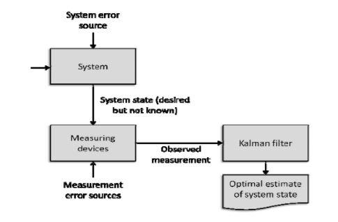
Fig.2.4.1 Typical Kalman filter application [26]
2.5 Using Landmarks for localization strategy
There are many techniques in which landmarks and triangulation of signals can be used as a part of navigational strategy. These methods are based on the accurate identification of objects and the features of the environment. The environmental features can be divided into four categories:
1. Active Beacons
These beacons are placed at fixed known locations in the environment. They transmit ultrasonic, IF, or RF signals in the environment, which can be received by the robot if it is in the proximity of these beacons.
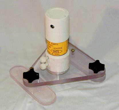
Fig.2.5.1 A single STROAB beams a vertically spread
laser signal while rotating at 3,000 rpm [27]
2. Artificial landmarks
These are specially designed objects or markers which are placed in the environment. The robot is programmed to detect these landmarks and calculate its position relative to these landmarks.
3. Natural Landmarks
Some of the distinguished features of the environment can be used a natural landmark. The natural landmarks can be detected with the help of sensors on the robot.
4. Prebuilt environmental models
Prebuilt environmental models can be used and the data from the sensors of the robot can be used to ascertain the accuracy of these models.
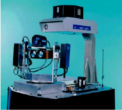
Fig.2.5.2. AECL’s natural landmark navigation system [27]
Of all the methods discussed above, the natural landmark method is the most flexible as there is no need to place artificial landmarks or beacons in the environment. However, it cannot be implemented successfully if the environment has low number of landmarks or the landmarks are such, that they do not provide any relevant information. With the advent of cheap digital cameras and progress in the field of computer vision, usage of digital cameras as a sensor to gather information about the environment has increased. When the cameras are used for performing SLAM, it is called as visual SLAM and EKF can be used for solving that problem. As EKF iteratively estimates the robots position, it is very effective in solving the SLAM problem. As the robot navigates through the environment, it gradually build’s up the map of the environment, as it encounters different waypoints [28]. Therefore, the localization problem can be solved by estimating the position of the robot and the position of the landmarks. The observation update step includes updating the landmarks and the joint co-variance matrix, every time an observation is made. The number of landmarks present in the environment leads to a quadratic increase in the extent of computations. However, the data from the landmarks is not observed by the robot regularly, neither it can be guaranteed that the landmarks will occur at fixed intervals. Hence, it is necessary to combine the positional information received from landmarks with odometry techniques [29, 30].
2.6 Summary
This chapter states the need for developing a robust and reliable localization strategy. A good navigational system is directly dependent on the localization system used by the robot. This chapter also describes how sensors can be used to tackle the problem of localization along with the problems one might face when using these sensors for localization. A brief overview of Kalman filter has been presented along with description of solutions based on probabilistic framework. In the last section, various advantages and disadvantages of using landmarks for navigation have been described.
Chapter 3 – 3pi and Odometry
The purpose of this chapter is to describe the odometric model used for the robot’s position calculation. The chapter further discusses the use of PID in conjunction with the odometric model to navigate to the given target following the shortest path possible to the target.
The content of this chapter is consisted of following parts:
- A brief overview of 3pi.
- Model for odometric position estimation.
- PID control of 3pi.
- Results of using odometry in conjunction with PID.
- Summary.
3.1 Overview of 3pi robot
The robot used for this entire research is the 3pi robot which is originally designed by ‘Pololu Robotics and Electronics’. The robot used in this particular research has been modified by ‘Auckland University of Technology’, such that there is an added ARM dev board, ‘mbed LPC1768’. This board is interfaced with the default AVR controller which was present on the 3pi in master slave configuration. The robot is also equipped with incremental rotary encoders, which provide pulses as each wheel moves. Some of the key specifications of the robot that are essential for obtaining proper odometric position estimation are as follows:
- RPM – 700
- Wheel diameter – 35mm
- Axle length – 96mm
- No. of pulses per revolution – 45
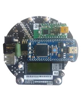
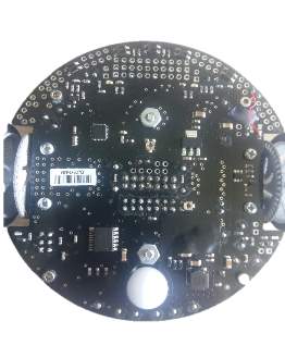
Fig.3.1.1 The top and the bottom view of the 3pi robot
3.2 The model for odometric position estimation
The position of the robot can be represented by the vector b = the axle length of the robot (i.e. the distance between the two wheels of the robot.)
Hence, we get the new updated position P’:
P’= x’y’θ’=P+ ∆s cosθ+∆θ2∆s sinθ+∆θ2∆θ=xyθ+ ∆s cosθ+∆θ2∆s sinθ+∆θ2∆θ (3.2.6)
From the relation for
(∆s;∆θ)of equations (3.2.4) and (3.2.5) we can get the basic equation for odometric update (applicable only for differential drive robots):
P’=fx,y,θ,∆sr, ,∆sl= xyθ+ ∆sr+∆sl2cosθ+∆sr-∆sl2b∆sr+∆sl2sinθ+∆sr-∆sl2b∆sr-∆slb (3.2.7)
As we know these odometric position updates present us with only a very rough estimation of where the robot actually is. Due to the integration errors of uncertainties in P the position error grows over time.
3.3 PID control of 3pi
In order to make the robot navigate from one point to another, the effectiveness of using only odometry along with PID was tested. In order to navigate the robot using the PID, it was necessary to calculate the PID constants of the robot. In order to do this, it was necessary to determine the speed at which the robot will be running. The full speed of the robot of 700 rpm was too fast and it was practically impossible to control the robot using PID at its full speed. Therefore, it was necessary to run the robot at a manageable speed. The header file developed by the 3pi robot community had a function to drive the motors at a particular speed, however the function didn’t provide us any information on the actual speed of the robot. Hence, the actual speed of the motors was calculated using a program, that simply counted the number of pulses received per second, which came out to be 149 for both the wheels.
For each differential drive robot, the change in heading is proportional to the wheel speed. Though in actuality the motor speed of the robot does not change equally for all pwm values supplied to the wheels, it has been assumed that it does in this research in order to simplify the calculations. Having stated that we can say that:
∆θ∆t =Arpr=-Alpl (3.2.8)
where,
∆θ∆t
is the change if heading angle over time and pr and pl are the pwm values which are provided to the right and left wheels respectively and Ar , Al are constants.
Though Ar and Al are different for each wheel, they are similar and have been assumed equal throughout the PID calculations. When the pwm signals are applied to the wheels at the same time we get:
∆θ∆t =Arpr-Alpl (3.2.9)
The figure mentioned at the bottom of the page represents the block diagram of the PID control used for the robot. F is the output of the PID calculation and is given by,
F=Kp.e+ Ki∫e∆t+ Kd∆e∆t (3.2.10)
Where, Kp and Ki are proportional and integral constants respectively e is the error in heading of the robot and ∆t is the frequency of the PID calculation. The pwm values that can be sent to the wheels of the robot range from 0 to 127. Hence, the output of the PID function i.e. F has been used to vary the pwm values sent to the wheels as follows:
if F >0 then pl=127 and pr=127-F
if F<0 then pr=127 and pl=127+F
if F=0 then pl=127 and pr=127
Estimating the values of A, Kp and Kd
From out earlier calculations we know that the speed of each motor of the robot is about 149 revolutions per second. From the robot’s dimensions and the resolutions of the wheel encoders it has been calculated that each wheel pulse causes the wheel to move about 2.373mm. Hence it can be calculated that id the difference between the pulses received from the wheels is 1 than the heading angle will change by about 1.4148 degrees.
∆θ∆t=149 ×1.414=210.686 degrees/sec=3.6791 rads/sec
So from equation (3.2.8),
∆θ∆t=Arpr
We get
Ar= 0.028969 as we have assumed
Ar=Al we conclude that
A=0.028969 and
A-1=34.5195.
In this experiment the PID control is implemented only when the heading error of the robot is below half a radian. If it is greater than half a radian, then the one motor runs at full speed while the other motor being stationary. So in order to estimate Kp considering a case when only proportional controller is implemented we get:
F= Kp.e
(3.2.11)
Considering the value of e=0.5 and F=127we get Kp=254
Assuming we want a critically damped condition where τ is the time response of the system we have, Kd= τ.Kp/(2-A-1) (3.2.12)
Ki=Kp24Kd+A-1 (3.2.13)
In order to get a system response time of 0.25 secs and substituting the previously derived values of A and Kp in the equation (3.2.12) and (3.2.13) we get Kd= -27.69 and Ki=25.4.
3.4 Program logic for navigation using PID
For navigation of the robot from one point to another, it is assumed that the robot will travel along the shortest path connecting the two points. The robot begins at a known position and also with a known heading angle. The target of the robot is specified in the form of x and y co-ordinates. Also the time period at which PID is calculated is one tenth of a second. The program to navigate to the target is implemented by keeping the track of the robot’s state. The state machine is implemented using the switch statements. The robot has four possible states i.e. start state, turn state, PID state and the stop state. The robot can only be in any one state at a time. The robot by defaults begins at the start state and should end up in the stop state as soon as it reaches its target.
Whenever the robot begins in the start state it checks for the distance to the target position. If this distance is less than 5cm it enters the stop state and stops both of its motors. However, if it is more than 5cms the robot enters the turn state. When in turn state the robot keeps its one wheel turned off and rotates the other one at full speed, depending on the direction in which the robot needs to turn to. The robot continues to turn till it either reaches its target or the error in the heading angle of the robot is less than 30 degrees. Once, the error in the heading angle is less than 30 degrees it enters into the PID state, where it uses the value of F calculated from the equation (3.2.10) to supply appropriate pwm values to the wheels of the robot.
3.5 Results for odometric navigation using the PID technique
The result shown below shows the robots path it thinks it follows according the odometric model described in section 3.2. The robot is running the above described program logic and the PID values calculated earlier. The numbers to the right in the picture show us the x and y co-ordinates of the point where, the robot thinks it is. It also shows the heading angle of the robot in degrees followed by the pulse count received by each wheel between every position update.
On the left hand side of the picture it shows the plot of the path followed by the robot from (0,0) to (2,2). As it is evident the robot takes a sharp turn from its origin as the error in heading angle is greater than 30 degrees. It enters into the PID state as soon as the error in the heading angle drops below 30 degrees and continues to follow the shortest path possible to the target.
These results prove that the odometric model used for the robot, which is described in the above section as well as the calculated PID values and program described above would have been sufficient for the navigation of the robot to the target had only if all the conditions would have been ideal. However, when tested it was found that the actual displacement of the robot in the actual environment did not agree with the calculated position using odometry. There may be several reasons for that, one of the reasons might be the inaccuracies in the diameters of the wheel or the wheels have slipped at some points resulting in inaccurate positioning.
Due to such disparities in the odmetric results and real life positioning there was a need to obtain a way to correct the position of the robot using data from the real environment in which the robot was in. The next chapter describes the method used for correcting the robots position using the data from the line sensors and its odometric calculation model.
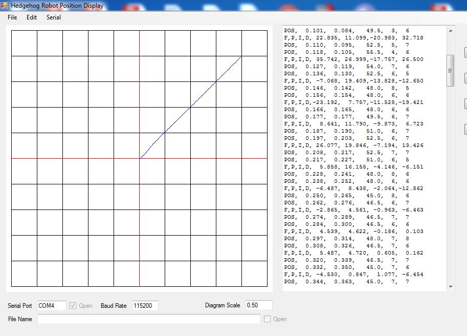
Fig.3.5.1 Results for navigation using PID and odometry
3.6 Summary
This chapter discusses the key features of the 3pi robot that needed to be taken into account for odometric calculations. The odometric model needed for performing the position calculation of the robot has been described. This chapter also mentions the fundamental equations needed for controlling the robot using PID method. The PID constants required for implementing PID on the robot have also been calculated.
The general program logic for navigation of the robot includes 4 states, namely the start state, stop state, turn state and the PID state. The robot switches through these states depending on the error in the heading angle of the robot and the current distance between its position and the target. When the program using this logic and calculated PID values was implemented on the robot, the results showed that, though the odometric calculations of the robot estimated it to be at the target the actual position of the robot in the real world differed from its odometric estimation. Though there may have been several factors responsible for this mismatch, the need for creating a more reliable localization method was felt in order to improve the odometric estimation. This novel method of position method using line sensors and odometry has been described in the following chapter.
Chapter 4 – A Novel Localization strategy
This chapter states the reasoning and inspiration behind using a localization strategy using line sensors and odometry. It also describes the method using which, the line sensors detected the lines and how reliable positional information was obtained from these sensors. The chapter also includes detailed program logic that has been used to program the robot. This chapter is divided into the following sections:
- Overview of the strategy
- Program logic
- Summary
4.1 Overview of the strategy
As per the discussion in the results section of the previous chapter, there was a need to develop a new localization scheme that would help the robot to correct its odometric estimation. As the robot was equipped with only line sensors, there was a need to come up with a way to use these line sensors in order to gain extra positional information of the robot. Hence an artificial environment was created in the form of a grid of lines. These parallel lines in the grid were spaced at a distance of 10cms from one another. After running some experiments, the ideal width of the lines so that they can be detected every time the line sensors cross over them, was determined to be 1cm. As for the odometric calculations, the robots position is assumed to be the geometric centre of the robot, the distance of each sensor from the robot’s geometric centre was calculated. The basic idea of using the grid of lines was inspired from the fact that the robot was using the x and y co-ordinate system for navigating in its environment. Hence, when a particular line sensor would cross over a line the position of that particular line sensor in the actual environment would be known. Once, the actual position of the robot’s sensor is known the actual co-ordinates of the geometric centre of the robot can be calculated, as its distance from the sensors is known. In this approach the robot was programmed to follow a circular path and it stored the positions of the sensors as they crossed the line. The complete program strategy and the calculations for the correction of odometric estimation of the robot will be discussed in the next section.
4.2 Program logic
As stated in the previous section, the robot is programmed to follow a circular trajectory by setting the speed of left wheel higher than the right wheel. As it goes around the environment, following its trajectory it detects the lines as it crosses them. The program can be broken down into the following logical steps:
1. Detecting the line:
A separate function is written in the code to detect the lines. It returns three different values i.e. one when it begins crossing the line, one when it has crossed the line and one to indicate when there is no change. The robot continuously polls the line sensors for the data, every 20ms. According to the values received from this function the GUI plots the location of the sensors, where they detected the lines, in the form of coloured dots.
2. Calculation of sensor position:
The odometric positional estimation of the sensors is calculated using the formulas below:
sensor x=x+0.050×cosh+0.03×sinh
sensor y=y+0.050×sinh+0.03×cosh
Where, sensor x and sensor y represent the x and y co-ordinates of the sensor and x, y represent the odometric co-ordinates of the robot. Once the sensor co-ordinates are obtained, the program determines the closest line to the sensor and concludes that it must have crossed that line. Once it has determined the line it has crossed, it stores the positional information of the sensor in an array dedicated to that line.
3. Sorting the points on the same line
Even after the points have been sorted such they are on the same line, it is necessary to sort them such that they lie on the opposite side of the line which is perpendicular to the line on which these points are detected, in order to calculate the slope connecting these two points on the opposite side.
4. Calculating the average of the points
As discussed in steps 2 and 3 points lying on a particular line will be sorted into two more groups i.e. points lying next to each other and points on the opposite side. The robots continuously sort the points as it goes around the environment and also maintains the positional average of each group of points.
5. Calculating the slope of line and correcting the heading angle
Once the robot has obtained sufficient number of points on either side of the line it calculates the slope of that line. The slope of this line indicates difference between the actual heading angle of the robot and the odometric heading angle of the robot.
Depending if the slope is negative or positive, it may be added or subtracted from the odometric heading of the robot.
6. Correcting the odometric positional co-ordinates of the robot
As the grid consists of only parallel and perpendicular lines, the robot can correct only a single co-ordinate based on the line which it has detected. To do this the, the position of the sensor is assumed to be at the centre of the line it crosses. The difference between the sensors actual position which is known depending on the line it has detected and its odometric position is calculated. This difference is then added to the corresponding co-ordinate of the robot’s odometric position.
All of the above steps can be repeated iteratively for each and every line it crosses over time as it travels around in a circle, thereby creating a more reliable and accurate localization scheme and further improving the odometric estimation of the robot’s position.
4.3 Summary
This chapter describes the inspiration behind using the described novel approach for correcting the odometric errors of the robot. By making the robot go around in circles it detects various lines using its line sensors. Whenever a line sensor detects a line it stores the current odometric position of the sensor in an array and sorts the points depending on their distance to various lines. Once the program has detected sufficient number of points it calculates the slope of the detected lines by using the positional information of the sensors which has been sorted previously. It then corrects the odometric heading angle of the robot using this calculated slope. In the next step it corrects the odometric co-ordinate of the robot by calculating the error between the odometric positional estimate of the sensor and the actual position of the sensor in the environment. The next chapter discusses the results that were achieved using this approach.
Chapter 5 – Results
This chapter discusses results obtained by running the program mentioned in the previous chapter on the 3pi robot. This chapter also describes the method in which the obtained results can be used in conjunction with the odometry model and the PID technique to accurately navigate to the target position. The chapter has been divided in the following sections:
- Discussion of test results
- Future use of the obtained results.
- Summary
5.1 Discussion of test results
For this particular test the correction in the heading angle and position co-ordinates was made when the robot encountered a vertical line i.e. the lines parallel to the Y axis. Initially the robot starts moving in its circular trajectory. In the odometry model of the robot the value of its starting points have been set to x = 0.2 and y = 0.4. These co-ordinates represent the distance in meters.
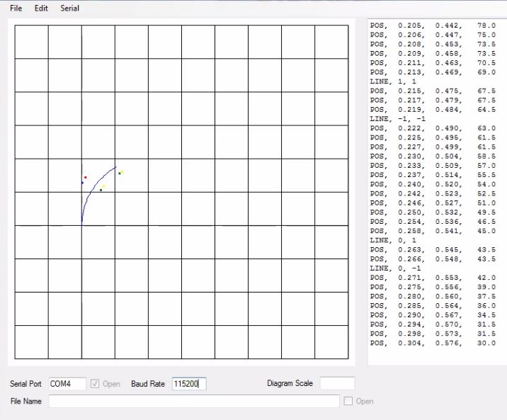
Fig.5.1.1 Result – 3pi start
In the Fig.5.1.2 the robot has travelled further along its trajectory and has started detecting the lines. Whenever the right most sensor of the robot crosses the line it is shown by green and yellow coloured dots on the GUI. Whereas, the red and yellow dots represent the crossing of line by the left most sensor of the robot. As it is apparent from the figure that the green and yellow dots are slightly off the vertical lines. However, what we expect to see is, as we cross across these vertical lines multiple times, the yellow and green coloured dots will me more clustered near the vertical lines.
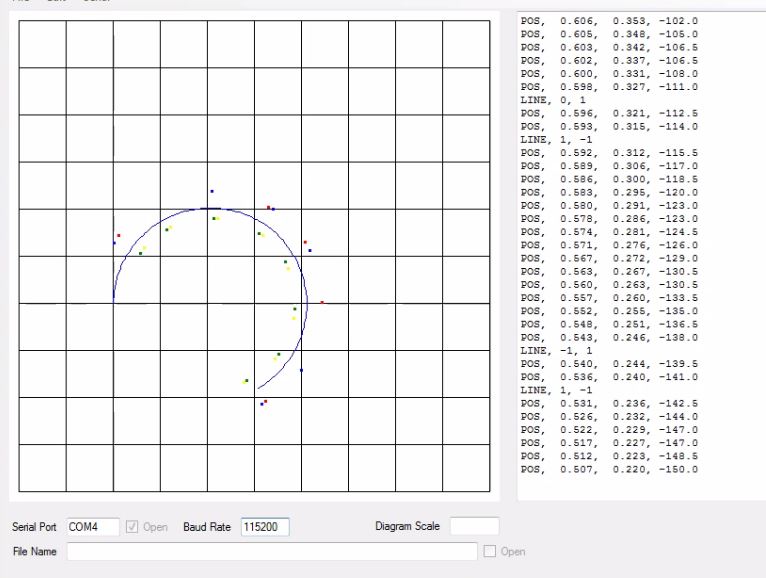
Fig.5.1.2 Result – 3pi traversed more than half of the circle
In Fig 5.1.3, it is evident that the robot has corrected its heading angle and its x co-ordinate as it passes through the point x = 0.430 and y = 0.194 as highlighted in the figure below. If compared with topmost reading highlighted in read, we can see that the robot has adjusted its heading angle, which is the number at the rightmost part of the reading by nearly 4 degrees. And also it has marginally adjusted its x co-ordinate. The reading highlighted in green represent the average x value of upper points along the line x=0.4, the average value of lower points along the same line, the current x co-ordinate of the rightmost sensor and the calculated slope of the line joining the upper and lower points in radians, respectively. It is difficult to notice the correction in values in the figure as the corrections are very subtle. However, when run for longer period of time the coloured dots start aligning to the lines.
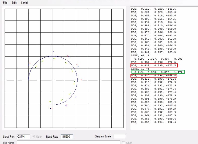
Fig.5.1.3 Result – 3pi correcting the odometry
When the robot is made to go around the lines few more times, what we are able to see is depicted in Fig.5.1.4. It is evident from this figure that the clustering of the points, which was slightly off the lines in the previous figures is much more centred around the x and y lines. Thus, the odometric model described in section 3.2, when combined with the localization approach discussed in chapter 4 has proved to be effective for creating more accurate position estimation of the 3pi robot in the real world environment.
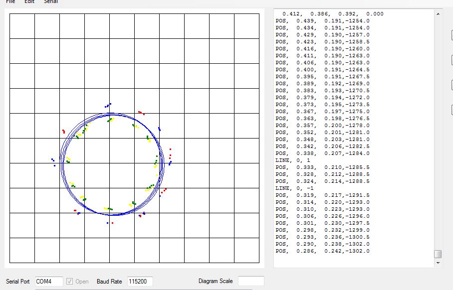
Fig 5.1.4 Result – Final output of the test
5.2 Future use of the obtained results
It is evident from the test results that the novel approach of using line sensors for odometry correction which, has been proposed in this paper has proven to be effective. The problem with navigating to a target position using only odometry and PID was that, there was no way for the robot to correct itself in case the wheels did not behave as exactly as predicted by the odometry model. However, if used in conjunction with the localization approach proposed in this paper it is possible to get impressive results as the robot can correct its odometric errors using line sensors.
Also, there is also a possibility to add more sensors such as laser range sensors or accelerometers and combine their data with line sensors and odometry, using Kalman filter to create a more robust localization module.
5.3 Summary
In this chapter it was established that the proposed localization approach has been proven to be effective in correcting the odometric position estimations of the robot. It has been demonstrated that this method is effective due to the fact that, as the robot goes around the lines constantly correcting itself, the actual position of the lines (indicated by the coloured dots) starts corresponding with the odometric lines (indicated by the GUI). There is also huge potential to further develop this localization approach by using it in conjunction with the data received from additional sensors and combining them using Kalman filter.
Chapter 6. Conclusion
From the very beginning the aim of this research was to create a more reliable localization strategy using only the data from the line sensors available on the robot. The results discussed in section 3.5 made it evident that there was a need to correct the odometric estimations of the robot from time to time. Even though these corrections may not appear to be very large, but due to the nature of the odometry these errors get accumulated over time. This results in a considerable error in position estimation of the robot, in its actual environment. The localization approach proposed in this paper was able to do just that. Every time the robot passes through the lines in the real environment it made subtle changes to the odometric positional estimation of the robot. When this process was repeated sufficient number of times, results showed that the lines in the real environment (indicated by the coloured dots in figures from section 5.1) started aligning with the odometric lines (indicated by the vertical and horizontal lines of GUI indicated in figures from section 5.1). Therefore, it can be concluded that this approach was successful in correcting the odometric position estimation of the robot.
References
[1] W. Hess, D. Kohler, H. Rapp, and D. Andor, Real-time loop closure in 2D LIDAR SLAM, 2016.
[2] H. Wang, H. Liu, H. Ju, and X. Li, “Improved Techniques for the Rao-Blackwellized Particle Filters SLAM,” in Intelligent Robotics and Applications: Second International Conference, ICIRA 2009, Singapore, December 16-18, 2009. Proceedings, M. Xie, Y. Xiong, C. Xiong, H. Liu, and Z. Hu, Eds., ed Berlin, Heidelberg: Springer Berlin Heidelberg, 2009, pp. 205-214.
[3] “A flexible and scalable SLAM system with full 3D motion estimation,” ed, 2011, p. 155.
[4] W. Burgard, A. B. Cremers, D. Fox, D. H, #228, hnel, et al., “The interactive museum tour-guide robot,” presented at the Proceedings of the fifteenth national/tenth conference on Artificial intelligence/Innovative applications of artificial intelligence, Madison, Wisconsin, USA, 1998.
[5] “The Office Marathon: Robust navigation in an indoor office environment,” ed, 2010, p. 300.
[6] “On the position accuracy of mobile robot localization based on particle filters combined with scan matching,” ed: IEEE, 2012, p. 3158.
[7] S. Zhang, L. Sun, Z. Chen, L. Zhang, and J. Liu, “A ROS-based smooth motion planning scheme for a home service robot,” 2015, pp. 5119-5124.
[8] “Monte Carlo Localization of Mobile Robot with Modified SIFT,” ed, 2009, p. 400.
[9] W. B. F Dellaert, D Fox, “Using the condensation algorithm for robust vision-based mobile robot localization,” presented at the Computer Vision and Pattern Recognition, 1999.
[10] J. J. L. P Elinas, “MCL: Monte-Carlo localization for mobile robots with stereo vision,” Proc. of Robotics: Science and Systems, 2005 2005.
[11] J. González, J. L. Blanco, C. Galindo, A. Ortiz-de-Galisteo, J. A. Fernández-Madrigal, F. A. Moreno, et al., “Mobile robot localization based on Ultra-Wide-Band ranging: A particle filter approach,” Robotics and Autonomous Systems, vol. 57, pp. 496-507, 1/1/2009 2009.
[12] C. Gamallo, C. V. Regueiro, P. Quintía, and M. Mucientes, “Omnivision-based KLD-Monte Carlo Localization,” Robotics and Autonomous Systems, vol. 58, pp. 295-305, 1/1/2010 2010.
[13] e. a. A. Gasparri, “Monte carlo filter in mobile robotics localization: a clustered evolutionary point of view,” Journal of Intelligent and Robotic Systems, vol. vol. 47(2), pp. 155-174, 2006.
[14] M.-H. Li, B.-R. Hong, Z.-S. Cai, S.-H. Piao, and Q.-C. Huang, “Novel indoor mobile robot navigation using monocular vision,” Eng. Appl. Artif. Intell., vol. 21, pp. 485-497, 2008.
[15] M. D’Souza, T. Wark, M. Karunanithi, and M. Ros, “Evaluation of realtime people tracking for indoor environments using ubiquitous motion sensors and limited wireless network infrastructure,” Pervasive and Mobile Computing, vol. 9, pp. 498-515, 8/1/August 2013 2013.
[16] D. Filliat and J. A. Meyer, “Map-based navigation in mobile robots: I. A review of localization strategies,” Cognitive Systems Research, vol. 4, pp. 243-282, 12 / 01 / 2003.
[17] Y. Elor and A. M. Bruckstein, “A “thermodynamic” approach to multi-robot cooperative localization,” Theoretical Computer Science, vol. 457, pp. 59-75, 10/26/26 October 2012 2012.
[18] e. a. R. Siegwart, Introduction to autonomous mobile robots: MIT press, 2011.
[19] e. a. E. Besada-Portas, “Localization of Non-Linearly Modeled Autonomous Mobile Robots Using Out-of-Sequence Measurements,” Sensors, vol. 12, pp. 2487-2518, 2012.
[20] R. C. Smith and P. Cheeseman, “On the representation and estimation of spatial uncertainly,” Int. J. Rob. Res., vol. 5, pp. 56-68, 1986.
[21] “Simultaneous map building and localization for an autonomous mobile robot,” ed, 1991, p. 1442.
[22] “Simultaneous localization and mapping (SLAM): part II,” IEEE Robotics & Automation Magazine, Robotics & Automation Magazine, IEEE, IEEE Robot. Automat. Mag., p. 108, 2006.
[23] H. Durrant-whyte and T. Bailey, Simultaneous localization and mapping: Part I vol. 13, 2006.
[24] B. Siciliano and O. Khatib, Springer Handbook of Robotics: Springer-Verlag New York, Inc., 2007.
[25] C. Cadena, L. Carlone, H. Carrillo, Y. Latif, D. Scaramuzza, J. Neira, et al., “Past, Present, and Future of Simultaneous Localization and Mapping: Toward the Robust-Perception Age,” Trans. Rob., vol. 32, pp. 1309-1332, 2016.
[26] I. R. N. Roland Siegwart, Introduction to Autonomous Mobile Robots. London, England: MIT press, 2004.
[27] H. E. Johann Borenstein, Liqiang Feng, Where am I? Sensors and methods for mobile robot positioning vol. 119, 1996.
[28] A. Chatterjee, O. Ray, A. Chatterjee, and A. Rakshit, “Development of a real-life EKF based SLAM system for mobile robots employing vision sensing,” Expert Systems With Applications, vol. 38, pp. 8266-8274, 1/1/2011 2011.
[29] M. Boccadoro, F. Martinelli, and S. Pagnottelli, “Constrained and quantized Kalman filtering for an RFID robot localization problem,” Autonomous Robots, vol. 29, pp. 235-251, 2010/11/01 2010.
[30] K. H. Yu, M. C. Lee, J. H. Heo, and Y. G. Moon, “Localization algorithm using a virtual label for a mobile robot in indoor and outdoor environments,” Artificial Life and Robotics, vol. 16, pp. 361-365, 2011/12/01 2011.
Cite This Work
To export a reference to this article please select a referencing stye below:
Related Services
View all


Related Content
All TagsContent relating to: "Technology"
Technology can be described as the use of scientific and advanced knowledge to meet the requirements of humans. Technology is continuously developing, and is used in almost all aspects of life.
Related Articles

DMCA / Removal Request
If you are the original writer of this dissertation and no longer wish to have your work published on the UKDiss.com website then please: