Image Segmentation on Integration with MATLAB and GPU
Info: 9870 words (39 pages) Dissertation
Published: 10th Dec 2019
Tagged: Information Technology
Abstract
Digital Image processing is the utilization of computer algorithms to implement image processing on images. Image Segmentation is a key innovation in image processing. It is the process of dividing a digital image into multiple segments or clusters. The principle motivation behind segmenting an image is to separate out the region of interest from the whole image. In digital image processing, diverse algorithms are utilized to perform image processing. As we have different region of interest for different application. None of the algorithm fulfills the worldwide application to give better outcome from computational perspective. The broad scope researchers had made a few strategies to manage the issue of image segmentation. Moreover, there are many general purpose algorithms have been developed in image segmentation over the time, in this project I have used Region-growing and K-mean clustering image segmentation algorithm. The combination of these two algorithm results into better segmentation results than the conventional methods. It represents the implementation of these two algorithms on MATLAB CPU for serial execution and implementation of same on GPU architecture for parallel execution. Parallel execution increases the processing speed of the processor. By integrating Matlab with Nvidia CUDA GPU, the computational complexity reduces; processing time reduces and speed increases. There is a performance improvement on using the CUDA GPU.
Chapter 1
Introduction
- Motivation
Accurate Image segmentation is one of the key issues in Computer Vision. Before any algorithm can be applied to an image it must be broken down into smaller major structural components, The way toward partitioning an image into segment locales or objects, in order to change the portrayal of an image into something that is simpler to break down with a specific end goal to get more data in the area of interest for an image which helps in comment of the object scene is alluded to as image segmentation. For instance, in radiation treatment arranging, radiologists need to figure the best way to apply radiation to a tumor while staying away from basic structures, for example, the eye and the kidney. To finish this errand, they obtain an arrangement of CT or MR pictures of the patient, physically follow the layouts of the basic structures on each picture, and utilize the subsequent shapes to fabricate 3D models. On the off chance that the image segmentation stage could be mostly mechanized, the time required for radiation treatment arranging would be lessened significantly.
- Background:
Image is a mix of small image focuses which are known as pixel. It is two-dimensional scattering of pixels. These two-dimensional pixels can be taken as an element of two genuine factors. Image segmentation is the handling of picture with the assistance of any scientific operations by working with any type of flag preparing considering the info is a picture. Thus, picture handling is the likewise the way toward enhancing and upgrading the picture lastly taking the helpful data from that picture. As, we will deal with Image segmentation which is one of the important advance in Image processing and assumes a key part in the investigation procedure of a picture. Image dividing into some significant locales relies upon surface, shading; movement, grayscale and profundity are the principle goal of picture division. The image segmentation operation is likewise used to recognize and find the essential items and its limits in pictures. There are different utilizations of Image processing which incorporates picture division additionally are Medical imaging; Content based picture recovery and Object discovery. Region Growing Algorithm and K-mean clustering Segmentation calculations are the calculations which are considered as best for image segmentation. While chipping away at the execution of segmentation calculations there are few issues with serial execution. Thus, parallel registering will be better for the cost sparing reason. Since in parallel calculation different figuring can be completed in the meantime while in serial just a single by one computation should be possible which takes additional time and more memory.
- Design Objective
The objective of this project is to implement the hybrid image segmentation algorithms (Region growing and K-mean Segmentation on MATLAB CPU and Integrating MATLAB with CUDA GPU.
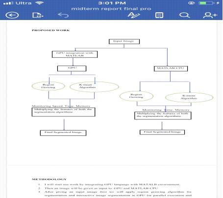
The above flow chart shows the objective or the methodology of my project. First of all an input image is taken then that input image is segmented using region growing algorithm and K-mean Image segmentation algorithm. Here, after running the memory, time and speed is measured. Then the final segmented image is achieved.
On the other side, the integration of GPU with MATLAB is done, here the hybrid of same segmentation algorithms are applied to CUDA GPU enabled MATLAB and segmentation is done. Again, memory, time and speed is measured and final image is achieved.
- METHODOLOGY
- Starting the work by integrating CUDA language with MATALB environment.
- Then an image will be given as input to CUDA GPU and MATLAB CPU
- After giving an input image first we will apply region growing algorithm for segmentation and interactive image segmentation in CUDA for parallel execution and only MATLAB for serial execution.
- The result of both the segmentation algorithms will be multiplied which will give final segmented image.
- While segmenting image time taken by system, memory consumed by both the systems (serial execution and parallel execution) will be monitored
- Based on which I will compare performance of CPU & GPU and will give objectives to improve the performance.
Chapter 2
2.1. Image Segmentation
Image segmentation is the process of segmenting or breaking a meaningless image into something more meaningful for different analysis purposes.
There are two objectives of Image Segmentation:
- The first objective is to break down the picture into parts for advance examination. In basic cases, the earth may be alright controlled so the division procedure dependably extricates just the parts that should be broke down further. For instance, in the part on shading, a calculation was exhibited for sectioning a human face from a shading video picture. The division is dependable, given that the individual’s garments or room foundation does not have indistinguishable shading parts from a human confront.
- The second objective of segmentation is to play out a difference in representation. The pixels of the picture must be sorted out into more elevated amount units that are either more significant or more efficient for advance investigation (or both). A basic issue is regardless of whether division can be performed for some different spaces utilizing general base up techniques that do not utilize any uncommon area learning.
Image segmentation algorithms should have following properties:
- Catch perceptually essential groupings or areas, which frequently reflect worldwide parts of the picture. Two focal issues are to give exact portrayals of what is perceptually essential, and to have the capacity to determine what a given division procedure does. We trust that there ought to be exact definitions of the properties of a subsequent division, keeping in mind the end goal to better comprehend the technique and to encourage the correlation of various methodologies.
- Be very proficient, running in time almost straight in the quantity of picture pixels. So as to be of functional utilize, we trust that division techniques ought to keep running at speeds like edge location or other low-level visual preparing procedures, which means almost direct time and with low steady factors. For case, a division method that keeps running at a few edges for every second can be utilized as a part of video handling applications.
Image segmentation is the division of an image into areas or classes which compares to various objects or parts of objects. Each pixel in an image is arranged into one of these classifications. For a few applications, for example, picture acknowledgment or compression, we can’t process the entire picture specifically for the reason that it is wasteful and strange. In this way, a few image segmentation calculations were proposed to section a picture before acknowledgment or compression. Picture division is to order or group and picture into a few sections (districts) as per the element of picture, for instance, the pixel esteem or the recurrence reaction. Up to now, heaps of picture division calculations exist and are widely connected in science and day by day life. As indicated by their division technique, we can around order them into area based division, information grouping, and edge-base division.
2.2. Segmentation Algorithms
The Image segmentation can be sorted into region based division, data clustering, and edge-base division. Region based division incorporates the seeded and unseeded locale developing calculations, the JSEG, and the quick segmentation calculations. Every one of them grow every region pixel by pixel in light of their pixel esteem or quantized esteem with the goal that each group has high positional connection.
- Edge based division: With this system, distinguished edges in an image are expected to speak to object boundaries, and used to recognize these objects. Indeed, even with idealize light, pixel based division brings about a predisposition of the extent of fragmented articles when the objects demonstrate varieties in their dim esteems .Darker items will turn out to be too little, brighter questions too expensive. The size varieties result from the way that the dark esteems at the edge of a protest change just step by step from the foundation to the protest esteem. No predisposition in the measure happens on the off chance that we take the mean of the protest and the foundation dark esteems as the limit. Nonetheless, this approach is just conceivable assuming all objects demonstrate a similar dark esteem or on the off chance that we apply distinctive limits for every protest. An edge based division approach can be utilized to stay away from an inclination in the extent of the portioned question without utilizing a complex thresholding plan. Edge-construct division is based with respect to the reality that the position of an edge is given by an extraordinary of the principal arrange subsidiary or a zero crossing in the second-arrange subsidiary.
- Gray scale image segmentation: The segmentation of picture raster information into associated locales of normal dark scale has long been viewed as a fundamental operation in picture investigation. In surface examination, simply this kind of division is conceivable after individual pixels in a picture have been named with a numeric classifier. In getting ready pictures for utilized as a part of geographic data frameworks (GIs) this division is generally trailed by the creation of a vector portrayal for each locale. The first calculation for division, created by Rosenfeld, depicted a two pass ‘successive calculation’ for the division of paired pictures. The key element of the Rosenfeld-pfaltz calculation is that the picture is raster-checked, first the forward heading, from upper left to base right, at that point in reverse. Amid the forward pass, every pixel is found an area name, in view of data looked over; the areas so divided may have pixels with more than one mark in that. Amid the regressive pass, a remarkable name is allocated to every pixel. Subsequently this work of art calculation can be portrayed as a two pass calculation.
- Model based segmentation: All division strategies examined so far use just neighborhood data. The human vision framework has the capacity to perceive protests regardless of the possibility that they are most certainly not totally spoke to. Clearly the data that can be assembled from nearby neighborhood administrators isn’t adequate to play out this errand. Rather particular information about the geometrical state of the articles is required, which would then be able to be contrasted and the neighborhood data. This line of reasoning prompts display based division. It can be connected if we know the correct state of the items contained in the picture.
- Color image segmentation: The human eyes have flexibility for the brilliance, which we can just distinguished handfuls of dark scale anytime of complex picture, yet can distinguish a huge number of hues. Much of the time, just use dim Level data cannot extricate the objective from foundation; we should by methods for shading data. In like manner, with the quickly change of PC handling abilities, the color image segmentation is being more worried by individuals. The shading picture division is likewise generally utilized as a part of numerous mixed media applications, for instance; keeping in mind the end goal to variably check huge quantities of pictures and video information in computerized libraries, they all should be arranged registry, arranging and capacity, the shading what’s more, surface are two most imperative highlights of data recovery in view of its substance in the pictures and video. In this way, the shading and surface division frequently utilized for ordering and administration of information; another case of sight and sound applications is the scattering of data in the system.
- Text segmentation: It is notable that content extraction, including content identification, restriction, division and acknowledgment is important for video auto-understanding. Examining content division, this is to isolate content pixels from complex foundation in the sub-pictures from recordings. Content division in video pictures is considerably more troublesome than that in examining pictures. Checking pictures for the most part has spotless and white foundation, while video pictures regularly have extremely complex foundation without earlier learning about the content shading. In spite of the fact that there have been a few effective frameworks of video content extraction, couple of analysts exceptionally contemplate content division in video pictures profoundly. The utilized methodologies could be arranged into two fundamental classifications: contrasts or best down) and similitude based (or base up) strategies. The to start with strategies depend on the foreground background differentiate.
- Region based division: Where an edge based method may endeavor to discover the question boundaries and after that find the object itself by filling them in, a region based procedure adopts the inverse strategy, by (e.g.) beginning amidst an object and afterward “developing” outward until the point when it meets the boundary limits.
- Data Clustering: Its one of the image segmentation method, cluster the primary idea of information bunching is to utilize the centroid to speak to each group and base on the closeness with the centroid of group to order. The work in the data clustering area typically falls into a number of broad categories.
- Strategy focused: Since bunching is a somewhat well known issue, it isn’t astounding that various strategies, for example, probabilistic procedures, remove based systems, otherworldly techniques, density-based methods, and dimensionality-diminishment based systems, are utilized for the grouping procedure. Each of these techniques has its own focal points and hindrances, and may function admirably in various situations and issue spaces. Certain sorts of information sorts, for example, high dimensional information, huge information, or gushing information have their own particular arrangement of difficulties and frequently require specific procedures.
- Watershed calculation: The primary objective of watershed calculation is to discover the watershed lines keeping in mind the end goal to isolate the particular regions. The watershed change is the procedure for choice for picture division in the field of logical morphology. We present a fundamental review of a couple of implications of the watershed change and the related progressive counts, and discuss diverse issues which consistently cause confuses in the written work. The need to perceive definition, calculation detail and figuring utilization is pointed out. Diverse representations are given which depict differentiates between watershed changes in perspective of different definitions or possibly executions.
2.3. Region Growing Segmentation Algorithm
The primary objective of division is to parcel a picture into locales. Some division strategies, for example, thresholding accomplish this objective by searching for the limits between locales in view of discontinuities in grayscale or shading properties. Area based division is a strategy for deciding the district straightforwardly.
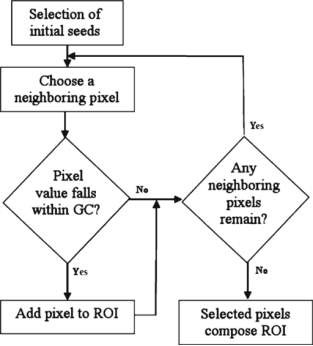
Region Growing segmentation process
The initial phase in locale developing is to choose an arrangement of seed focuses. Seed point determination depends on some client basis (for instance, pixels in a specific grayscale extend, pixels equally divided on a lattice, and so forth.). The underlying locale starts as the correct area of these seeds. The locales are then developed from these seed focuses to contiguous focuses relying upon a district enrollment standard.
Advantages of Region-Growing Algorithm:
- Region growing strategy can accurately isolate the districts that have similar properties we characterize.
- Region Growing methods can give the first pictures which have clear edges with great division comes about.
- The idea is straightforward. We just need few seed focuses to speak to the property we need, at that point develop the area.
- We can decide the seed focuses and the criteria we need to make.
- We can pick the different criteria in the meantime.
2.4. K-mean clustering:
Image segmentation is the order of an image into various gatherings. Many investigates have been done in the range of image segmentation utilizing clustering. There are distinctive strategies and a standout amongst the most mainstream techniques is K-mean clustering algorithm… K – Implies clustering calculation is an unsupervised calculation and it is utilized to portion the interested area from the background.
Be that as it may, before applying K – implies calculation, first incomplete extending upgrade is connected to the image to enhance the nature of the image. Subtractive clustering technique is information grouping strategy where it creates the centroid in light of the potential estimation of the information focuses. So subtractive group is utilized to produce the underlying focuses and these focuses are utilized as a part of k-implies calculation for the division of picture. At that point at long last media filter is connected to the sectioned image to expel any undesirable area from the image.
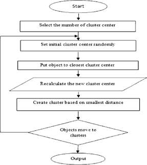
K-mean clustering algorithm process
- K-mean clustering is efficient and fast. It computes result at 0 (tkn). Where n is number of objects or points, k is number of clusters and t is number of iterations. K-means clustering can be applied to machine learning or data mining.
Chapter 3
3.1. Graphical Processing Unit
An illustrations preparing unit (GPU) is a specific electronic circuit intended to quickly control and adjust memory to quicken the production of pictures in a casing cradle expected for yield to a show gadget. GPUs are utilized as a part of implanted frameworks, cell phones, PCs, workstations, and amusement comforts. Current GPUs are extremely proficient at controlling PC illustrations and picture preparing, and their very parallel structure makes them more effective than broadly useful CPUs for calculations where the handling of extensive pieces of information is done in parallel. In a PC, a GPU can be available on a video card, or it can be installed on the motherboard or—in specific An outer GPU is an illustrations processor situated outside of the lodging of the PC. Outer illustrations processors are some of the time utilized with smart phones. Tablets may have a significant measure of RAM and an adequately effective focal preparing unit (CPU), yet frequently do not have an intense illustrations processor, and rather have a less capable however more vitality productive on-board designs chip. On-board illustrations chips are regularly not sufficiently capable for playing the most recent diversions, or for other graphically escalated assignments, for example, altering video. CPUs—on the CPU die.
3.2. GPU’s With MATLAB
The main purpose of GPU computing in MATLAB is to speed up the application.
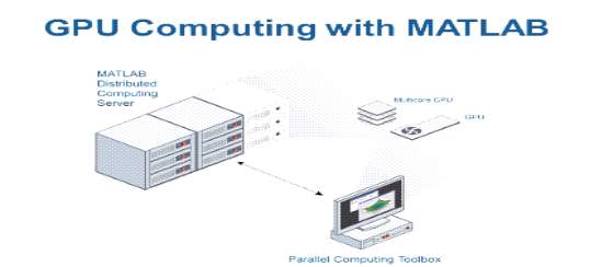
The above figure depicts the GPU computing with MATLAB.
Parallel Computing Toolbox empowers the MATLAB program to utilize the PC’s Graphic processing unit (GPU) for grid operations. By and large, execution in the GPU is quicker than in the CPU, so this component may offer enhanced execution. The enhancement in the execution of the GPU by doing some calculations in single accuracy rather than twofold exactness. In CPU calculations, then again, we don’t get this change when changing from twofold to single exactness. The reason is that most GPU cards are intended for realistic show, requesting high single accuracy execution.
Initially used to quicken designs rendering, GPUs are presently progressively connected to logical computations. Dissimilar to a customary CPU, which incorporates close to a modest bunch of centers, a GPU has a hugely parallel cluster of whole number and drifting point processors, and also devoted, fast
memory. A run of the mill GPU contains several these littler processors. These processors can be utilized to incredibly accelerate specific sorts of utilizations.
How GPU improves the performance?
- While changing over MATLAB code to keep running on the GPU, it is best to begin with MATLAB code that as of now performs well. While the GPU and CPU have distinctive execution attributes, the general rules for composing great MATLAB code likewise enable to compose great MATLAB code for the GPU.
- The initial step is quite often to profile the CPU code. The lines of code that the profiler indicates taking the most time on the CPU will probably be ones that you should focus on when you code for the GPU.
- It is most effortless to begin changing over the code utilizing MATLAB worked in capacities that help gpuArray information. These capacities take gpuArray inputs, perform counts on the GPU, and return gpuArray output.
- A rundown of the MATLAB capacities that help gpuArray information is found in Run Built-In Functions on a GPU. As a rule these capacities bolster similar contentions and information sorts as standard MATLAB capacities that are ascertained in the CPU. Any constraints in these capacities for gpuArrays are portrayed in their summon line help (e.g., help gpuArray/qr).
- On the off chance that every one of the capacities that you need to utilize are bolstered on the GPU, running code on the GPU might be as basic as calling gpuArray to exchange enter information to the GPU, and calling accumulate to recover the yield information from the GPU when wrapped up.
- By and large, we may need to vectorize the code, supplanting circled scalar operations with MATLAB network and vector operations. While vectorizing is by and large a decent practice on the CPU, it is generally basic for accomplishing elite on the GPU.
3.3. GPU Acceleration
A GPU can accelerate an application if it fits both of the following criteria:
- Computationally intensive—the time spent on calculation essentially surpasses the time spent on exchanging information to and from GPU memory.
- Massively parallel—the calculations can be separated down into hundreds or thousands of autonomous units of work.
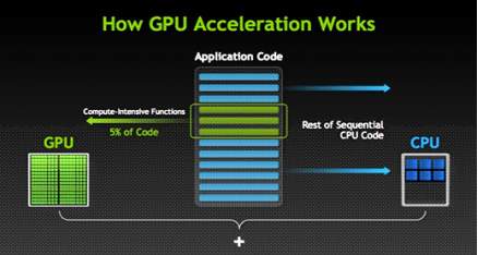
GPU acceleration
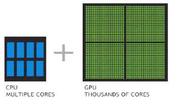
- GPU-accelerated registering offloads computer-intensive parts of the application to the GPU, while the rest of the code still keeps running on the CPU. From a client’s point of view, applications basically run significantly speedier.
- A straightforward approach to comprehend the distinction between a GPU and a CPU is to think about how they process errands. A CPU comprises of a couple of cores enhanced for successive serial preparing while a GPU has a greatly parallel engineering comprising of thousands of littler, more effective cores intended for dealing with numerous assignments at the same time.
- A decent general guideline is that your concern might be a solid match for the GPU on the off chance that it is:
- Hugely parallel: The calculations can be separated into hundreds or thousands of autonomous units of work. You will see the best execution when the majority of the centers are kept occupied with, misusing the inalienable parallel nature of the GPU. Apparently basic, vectorized MATLAB computations on exhibits with a huge number of components regularly can fit into this class.
- Computationally escalated: The time spent on calculation fundamentally surpasses the time spent on exchanging information to and from GPU memory. Since a GPU is connected to the host CPU by means of the PCI Express transport, the memory get to is slower than with a conventional CPU. This implies your general computational speedup is constrained by the measure of information move that happens in your calculation.
Chapter 4
4.1. What is CUDA?
CUDA stands for computer unified device architecture. CUDA has the only ecosystem with all of the libraries necessary for technical computing.
CUDA is a parallel registering stage and application programming interface (API) show made by Nvidia. It permits programming designers and programming architects to utilize a CUDA-empowered illustrations preparing unit (GPU) for universally useful handling – an approach named GPGPU (General-Purpose figuring on Graphics Processing Units). The CUDA stage is a product layer that gives guide access to the GPU’s virtual direction set and parallel computational components, for the execution of process kernels.
The CUDA stage is intended to work with programming dialects, for example, C, C++, and Fortran. This availability makes it less demanding for experts in parallel programming to utilize GPU assets, rather than earlier APIs like Direct3D and OpenGL, which required propelled aptitudes in designs programming. Likewise, CUDA bolsters programming systems, for example, OpenACC and OpenCL. When it was first presented by Nvidia, the name CUDA was an acronym for Compute Unified Device Architecture; however Nvidia in this manner dropped the utilization of the acronym.
The designs preparing unit (GPU), as a specific PC processor, addresses the requests of constant high-determination 3D illustrations register concentrated undertakings. By 2012, GPUs had advanced into profoundly parallel multi-center frameworks permitting exceptionally proficient control of vast squares of information. This plan is more powerful than universally useful focal handling unit (CPUs) for calculations in circumstances where preparing extensive pieces of information is done in parallel, for example, push-reliable most extreme stream calculation quick sort calculations of huge records two-dimensional quick wavelet change sub-atomic progression reenactments.
The accompanying advances depict the CUDA Kernel general work process
- Use aggregated PTX code to make a CUDA Kernel protest, which contains the GPU executable code.
- Set properties on the CUDA Kernel question control its execution on the GPU.
- Call feval on the CUDA Kernel with the expected contributions, to run the part on the GPU.
- CUDA empowers coordinate GPU programming.
- Parallel portions run single program in many strings on the gadget.
- GPU strings are amazingly light weight.
4.2. CUDA Programming Model:
CUDA consist of sets of C language extensions and a run time library that provides Application program interfaces to control the GPU. Therefore CUDA programming model allows programming to better exploit the parallel power of GPU for general purpose computing.
Although MATLAB is used for mathematical calculation but here we are using it for image processing and integrating it with CUDA programming model for some parallel processing. I am using MATLAB 2016 for my parallel processing.
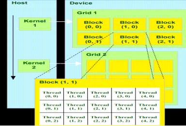
CUDA Programming Model
- A kernel is executed by group of thread blocks.
- A thread block is a back of thread that can be operated with each other by:
- Sharing data through shared memory
- Synchronizing their execution.
- Threads from different block cannot cooperate.
- Write a solitary strung program parameterized regarding the string ID.
- Use the string ID to choose a subset of the information for preparing, and to settle on control stream choices.
- Launch various strings, with the end goal that the troupe of strings forms the entire informational collection.
MATLAB Code that follows above step can be written as:
% 1. Create CUDAKernel object.
k = parallel.gpu.CUDAKernel(‘myfun.ptx’,’myfun.cu’,’entryPt1′);
% 2. Set object properties.
k.GridSize = [8 1];
k.ThreadBlockSize = [16 1];
% 3. Call feval with defined inputs.
g1 = gpuArray(in1); % Input gpuArray.
g2 = gpuArray(in2); % Input gpuArray.
result = feval(k,g1,g2);
4.3. CUDA GPU
The CUDA GPU processing can be explained as:
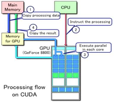
CUDA is a parallel computing platform and application programming interface (API) model created by Nvidia. It allows software developers and software engineers to use a CUDA-enabled graphics processing unit (GPU) for general purpose processing
Chapter 5
5.1. CPU Vs GPU
Not at all like a conventional CPU, which incorporates close to a modest bunch of cores, has a GPU had a greatly parallel cluster of number and floating point processors, and committed rapid memory. A regular GPU contains several these littler processors.
Comparison of number of chores on CPU system and GPU system.
The significantly expanded throughput made conceivable by a GPU, in any case, includes some major disadvantages. Initially, memory gets to turns into a substantially more likely bottleneck for your figuring. Information must be sent from the CPU to the GPU before
Estimation and after that recovered from it a short time later. Since a GPU is appended to the host CPU by means of the PCI Express bus, the memory get to is slower than with a customary CPU.1 this implies your general computational speedup is constrained by the measure of information move that happens in your algorithm. Second, programming for GPUs in C or FORTRAN requires an alternate mental model and a range of abilities that can be troublesome and tedious to secure. Moreover, should invest energy tweaking your code for your particular GPU to improve your applications for peak execution.
Chapter 6
Serial Execution
Implementation on MATLAB CPU
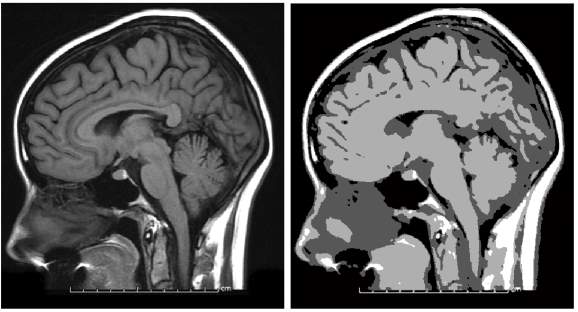
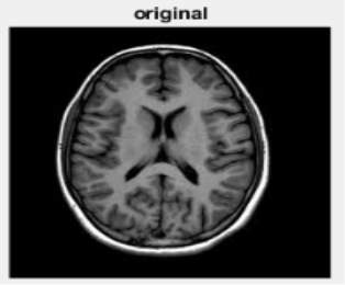
In this project I took a brain image as an original image, I applied k-mean and region-growing algorithm on the image. I calculated the elapsed time and the memory used by both of these algorithms in MATLAB CPU and then MATLAB GPU.
- MATLAB Code for Region Growing Segmentation Algorithm: (Serial)
tic
I = imread(‘C:UsersLenovoDesktopswatii.jpg’); % Loading Image
I2 = im2double(I)
x=158; y=130;
J = regiongrowing(I2,x,y,0.2);
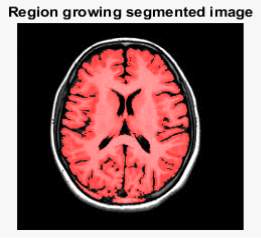
figure, imshow(I2+J); title(‘Region growing segmented image’)
cputime
memory
toc
Where J= regiongrowing(I2, x,y,0.2) is the region growing function which is called and explains:
function J=regiongrowing(I,x,y,reg_maxdist)
if(exist(‘reg_maxdist’,’var’)==0), reg_maxdist=0.2; end
if(exist(‘y’,’var’)==0), figure, imshow(I,[]); [y,x]=getpts; y=round(y(1)); x=round(x(1)); end
% Output
J = zeros(size(I));
% Dimensions of input image
Isizes = size(I);
reg_mean = I(x,y); % The mean of the segmented region
reg_size = 1; % Number of pixels in region
% Free memory to store neighbours of the (segmented) region
neg_free = 10000; neg_pos=0;
neg_list = zeros(neg_free,3);
pixdist=0; % Distance of the region newest pixel to the regio mean
% Neighbor locations (footprint)
neigb=[-1 0; 1 0; 0 -1;0 1];
while(pixdist<reg_maxdist&®_size<numel(I))
% Add new neighbors pixels
for j=1:4,
% Calculate the neighbour coordinate
xn = x +neigb(j,1); yn = y +neigb(j,2);
% Check if neighbour is inside or outside the image
ins=(xn>=1)&&(yn>=1)&&(xn<=Isizes(1))&&(yn<=Isizes(2));
% Add neighbor if inside and not already part of the segmented area
if(ins&&(J(xn,yn)==0))
neg_pos = neg_pos+1;
neg_list(neg_pos,:) = [xn yn I(xn,yn)]; J(xn,yn)=1;
end
end
% Add a new block of free memory
if(neg_pos+10>neg_free), neg_free=neg_free+1000; neg_list((neg_pos+1):neg_free,:)=0; end
dist = abs(neg_list(1:neg_pos,3)-reg_mean);
[pixdist, index] = min(dist);
J(x,y)=2; reg_size=reg_size+1;
% Calculate the new mean of the region
reg_mean= (reg_mean*reg_size + neg_list(index,3))/(reg_size+1);
% Save the x and y coordinates of the pixel (for the neighbour add proccess)
x = neg_list(index,1); y = neg_list(index,2);
% Remove the pixel from the neighbour (check) list
neg_list(index,:)=neg_list(neg_pos,:); neg_pos=neg_pos-1;
end
% Return the segmented area as logical matrix
J=J>1;
Region Growing Segmented Image:
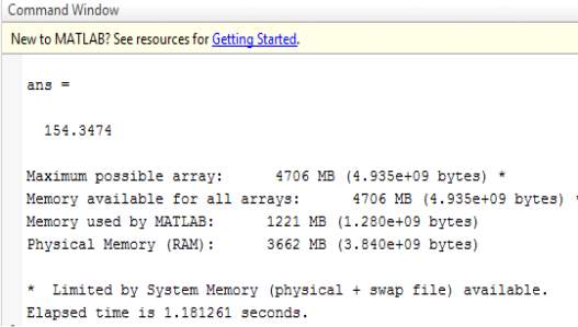
Measured Time and Memory on MATLAB Command Window:
- MATLAB Code for K – Mean Segmentation Algorithm: (Serial)
clc
clear all
close all
tic
I = im2double(imread(‘C:UsersLenovoDesktopswatii.jpg’)); % Loading Image
F = reshape(I,size(I,1)*size(I,2),3); % If we take color image as an input
%% K-means
K = 6; % Optional Cluster Numbers – can choose according to input image
CENT = F( ceil(rand(K,1)*size(F,1)) ,:); % We need to define the centres of cluster
DAL = zeros(size(F,1),K+2); % Distances and Labels
KMI = 10; % how many time K-means will Iterate
for n = 1:KMI
for i = 1:size(F,1)
for j = 1:K
DAL(i,j) = norm(F(i,:) – CENT(j,:));
end
[Distance, CN] = min(DAL(i,1:K));
DAL(i,K+1) = CN;
DAL(i,K+2) = Distance;
end
for i = 1:K
A = (DAL(:,K+1) == i);
CENT(i,:) = mean(F(A,:));
if sum(isnan(CENT(:))) ~= 0
NC = find(isnan(CENT(:,1)) == 1);
for Ind = 1:size(NC,1)
CENT(NC(Ind),:) = F(randi(size(F,1)),:);
end
end
end
end
toc
X = zeros(size(F));
for i = 1:K
idx = find(DAL(:,K+1) == i);
X(idx,:) = repmat(CENT(i,:),size(idx,1),1);
end
T = reshape(X,size(I,1),size(I,2),3);
%% Output images/segmented image after applying k-means clustering
figure()
imshow(I); title(‘original’)
figure()
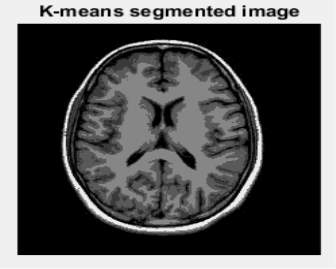
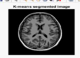
imshow(T); title(‘K-means segmented image’)
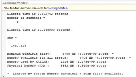
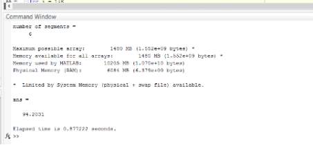
disp(‘number of segments =’); disp(K)
toc
cputime
memory
K-Mean Segmented Image:
Measured Time and Memory on MATLAB Command Window:
- MATLAB Code for Hybrid Region Growing and K – Mean Segmentation Algorithm: (Serial)
clc
clear all
close all
tic
I = im2double(imread(‘C:UsersLenovoDesktopswatii.jpg’)); % Loading Image
F = reshape(I,size(I,1)*size(I,2),3); % If we take color image as an input
%% K-means
K = 6; % Optional Cluster Numbers – can choose according to input image
CENT = F( ceil(rand(K,1)*size(F,1)) ,:); % We need to define the centres of cluster
DAL = zeros(size(F,1),K+2); % Distances and Labels
KMI = 10; % how many time K-means will Iterate
for n = 1:KMI
for i = 1:size(F,1)
for j = 1:K
DAL(i,j) = norm(F(i,:) – CENT(j,:));
end
[Distance, CN] = min(DAL(i,1:K));
DAL(i,K+1) = CN;
DAL(i,K+2) = Distance;
end
for i = 1:K
A = (DAL(:,K+1) == i);
CENT(i,:) = mean(F(A,:));
if sum(isnan(CENT(:))) ~= 0
NC = find(isnan(CENT(:,1)) == 1);
for Ind = 1:size(NC,1)
CENT(NC(Ind),:) = F(randi(size(F,1)),:);
end
end
end
end
X = zeros(size(F));
for i = 1:K
idx = find(DAL(:,K+1) == i);
X(idx,:) = repmat(CENT(i,:),size(idx,1),1);
end
T = reshape(X,size(I,1),size(I,2),3);
%% Output images/segmented image after applying k-means clustering
figure()
imshow(I); title(‘original’)
figure()
imshow(T); title(‘K-means segmented image’)
disp(‘number of segments =’); disp(K)
%%cputime
%%memory
%%toc
%%region growing
I2 = im2double(T)
x=178; y=150;
J = regiongrowing(I2,x,y,0.2);
figure, imshow(I2+J); title(‘Segmented image after applying k-means and region growing’)
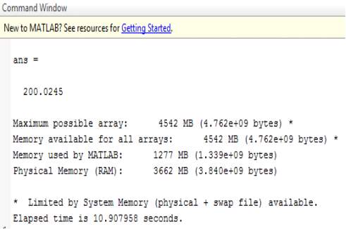
cputime
memory
toc
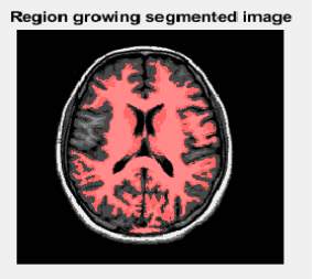
Hybrid Segmented Image:
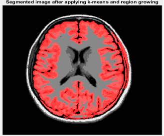
The figure show hybrid segmented which means , first k mean segmentation algorithm has been applied than the k mean segmented image is taken as input image for region growing segmentation algorithm.
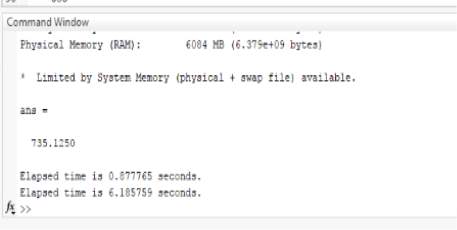
Measured Time and Memory on MATLAB Command Window:
Chapter 7
Parallel Execution
Implementation on MATLAB GPU
- K-MEAN SEGMENTATION ON INTEGRATING MATLAB CUDA GPU
CODE:
clc
clear all
close all
tic
I = im2double(imread(‘download.jpg’)); % Loading Image
F = reshape(I,size(I,1)*size(I,2),3); % If we take color image as an input
%% K-means
K = 6; % Optional Cluster Numbers – can choose according to input image
CENT = F( ceil(rand(K,1)*size(F,1)) ,:); % We need to define the centres of cluster
DAL = zeros(size(F,1),K+2); % Distances and Labels
KMI = 10; % how many time K-means will Iterate
% this array needs to be 1-D to hold the data coming
% from GPU (because in CUDA we use 1-D array)
DAL_host = zeros(size(F,1)*(K+2),1);
gpu_DAL = gpuArray(DAL_host); %this is the DAL array in CUDA memory in 1-D
% we need to reshape the F array before uploading in GPU memory
dev_F = gpuArray(reshape(F.’,1,[]));
% CUDA configuration, 1st compile the kernel (only once is needed)
% then make a MATLAB object of this kernel
% system(‘nvcc -ptx distLabelCalc.cu’);
k = parallel.gpu.CUDAKernel(‘distLabelCalc.ptx’, ‘distLabelCalc.cu’);
% we call the kernel with 5 CUDA blocks of 256 threads in each one!
% this is equivalent with distLabelCalc<<< 5, 256>>>(….);
k.ThreadBlockSize = [256, 1, 1];
k.GridSize = [5, 1];
for n = 1:KMI
% the CENT array is modified in each iteration so we need to
% refresh the GPU memory. Notice that it also needs to be reshaped in
% 1-D row-major format
dev_CENT = gpuArray(reshape(CENT.’,1,[]));
% this command launches the CUDA kernel with parameteres like above!
% we need to set the dev_DAL as the return array
gpu_DAL = feval(k, dev_F, gpu_DAL, dev_CENT, size(F,1), K);
% the gpu_DAL needs to return in CPU, the gather() command offloads it
% from GPU->CPU like cudaMemcpy() in CUDA
DAL_host = gather(gpu_DAL);
%IMPORTANT: reshape it in original dimensions of DAL -> (50400×8)
DAL = reshape(DAL_host, 8, size(F,1))’;
% now make the rest of checks in CPU, results from CENT will be
% uploaded in GPU in next iteration
for i = 1:K
A = (DAL(:,K+1) == i);
CENT(i,:) = mean(F(A,:));
if sum(isnan(CENT(:))) ~= 0
NC = find(isnan(CENT(:,1)) == 1);
for Ind = 1:size(NC,1)
CENT(NC(Ind),:) = F(randi(size(F,1)),:);
end
end
end
end
X = zeros(size(F));
for i = 1:K
idx = find(DAL(:,K+1) == i);
X(idx,:) = repmat(CENT(i,:),size(idx,1),1);
end
T = reshape(X,size(I,1),size(I,2),3);
%% Output images/segmented image after applying k-means clustering
figure()
imshow(I); title(‘original’)
figure()
imshow(T); title(‘K-means segmented image’)
disp(‘number of segments =’); disp(K)
cputime
toc
%memory
K-Mean Segmented Image on GPU:
Measured Time and Memory on MATLAB Command Window Integration with CUDA GPU:
- K-Mean and Region Growing Segmentation on Integrating MATLAB CUDA GPU
Code:
function J=regiongrowingGPU(I,x,y,reg_maxdist)
if(exist(‘reg_maxdist’,’var’)==0), reg_maxdist=0.2; end
if(exist(‘y’,’var’)==0), figure, imshow(I,[]); [y,x]=getpts; y=round(y(1)); x=round(x(1)); end
% Output
Jtemp = zeros(size(I));
J = zeros(size(I));
% Dimensions of input image
Isizes = size(I);
reg_mean = I(x,y); % The mean of the segmented region
reg_size = 1; % Number of pixels in region
% Free memory to store neighbours of the (segmented) region
neg_free = 10000;
neg_pos=0;
neg_list = zeros(neg_free,3);
d_neg_list = zeros(neg_free,1,’gpuArray’);
pixdist=0; % Distance of the region newest pixel to the regio mean
% Neighbor locations (footprint)
neigb=[-1 0; 1 0; 0 -1;0 1];
%this kernel is a faster way to update the neg_list array in GPU
k = parallel.gpu.CUDAKernel(‘arrayAssign.ptx’, ‘arrayAssign.cu’);
k.ThreadBlockSize = [1, 1, 1];
k.GridSize = [1, 1];
%tic
while(pixdist<reg_maxdist&®_size<numel(I))
start = neg_pos;
% Add new neighbors pixels
for j=1:4,
% Calculate the neighbour coordinate
xn = x +neigb(j,1);
yn = y +neigb(j,2);
% Check if neighbour is inside or outside the image
ins=(xn>=1)&&(yn>=1)&&(xn<=Isizes(1))&&(yn<=Isizes(2));
% Add neighbor if inside and not already part of the segmented area
if(ins&&(Jtemp(xn,yn)==0))
neg_pos = neg_pos+1;
neg_list(neg_pos,:) = [xn yn I(xn,yn)];
Jtemp(xn,yn)=1;
end
end
% update in GPU using an assign kernel
d_neg_list = feval(k, d_neg_list, neg_list(start+1,3), neg_list(start+2,3), neg_list(start+3,3),…
neg_list(start+4,3), start);
% Add a new block of free memory
if(neg_pos+10>neg_free)
neg_free=neg_free+1000;
neg_list((neg_pos+1):neg_free,:)=0;
end
% now in GPU
dist = abs(d_neg_list(1:neg_pos)-reg_mean);
[d_pixdist, d_index] = min(dist);
% take values from GPU memory back to host Matlab
pixdist = gather(d_pixdist);
index = gather(d_index);
neg_list(index,3)= gather( d_neg_list(index) );
d_neg_list(index) = d_neg_list(neg_pos);
Jtemp(x,y)=2;
reg_size=reg_size+1;
% Calculate the new mean of the region
reg_mean= (reg_mean*reg_size + neg_list(index,3))/(reg_size+1);
% Save the x and y coordinates of the pixel (for the neighbour add proccess)
x = neg_list(index,1);
y = neg_list(index,2);
% Remove the pixel from the neighbour (check) list
neg_list(index,:)=neg_list(neg_pos,:);
neg_pos=neg_pos-1;
end
%toc
% Return the segmented area as logical matrix
J=Jtemp>1;
Array Design:
__global__ void arrayAssign(double *input, double v1, double v2, double v3, double v4, int start)
{
// the global index of each thread, we need it to have the threads started in
// correct positions
//int gid = blockDim.x*blockIdx.x + threadIdx.x;
// the local index inside a CUDA block, useful for loading CENT data in local memory
int tid = threadIdx.x;
if(tid==0)
{
input[start] = v1;
input[start+1] = v2;
input[start+2] = v3;
input[start+3] = v4;
}
}
Distance Label:
__global__ void distLabelCalc(const double *F, double *DAL, const double *CENT, int N, int K)
{
// the global index of each thread, we need it to have the threads started in
// correct positions
int gid = blockDim.x*blockIdx.x + threadIdx.x;
// the local index inside a CUDA block, useful for loading CENT data in local memory
int tid = threadIdx.x;
// shared memory is useful when some data need to be reused many times
// so the threads will accees them on-chip memory (many times faster!)
__shared__ double l_CENT[18];
if (tid<K * 3)
l_CENT[tid] = CENT[tid];
//IMPORTANT: synchronize threads inside a block so all threads can see the shared l_CENT array updated
__syncthreads();
// begin each CUDA threads from its global position, then make steps according to
// total number of active threads
for (int i = gid; i<N; i += blockDim.x*gridDim.x)
{
// fetch the 3 dimensions of each points from global memory!
// have in mind that array is 1-D (unlike MATLAB)
double f1 = F[i * 3];
double f2 = F[i * 3 + 1];
double f3 = F[i * 3 + 2];
double CN; //some helper variables for the k-means search
double minDist = 100;
double newDist;
for (int j = 0; j<K; j++)
{
// take the square of difference between each point and the K centers
// this part is doing the DAL(i,j) = norm(F(i,:) – CENT(j,:)); from MATLAB
double d1 = (l_CENT[j * 3] – f1)*(l_CENT[j * 3] – f1);
double d2 = (l_CENT[j * 3 + 1] – f2)*(l_CENT[j * 3 + 1] – f2);
double d3 = (l_CENT[j * 3 + 2] – f3)*(l_CENT[j * 3 + 2] – f3);
newDist = sqrt(d1 + d2 + d3);
// upload our global memory with each distance
DAL[i*(K + 2) + j] = newDist;
// choose the closer Center! and keep the index of it
// in MATLAB is [Distance, CN] = min(DAL(i,1:K));
if (newDist < minDist)
{
CN = (double)j + 1;
minDist = newDist;
}
}
//update the global memory
DAL[i*(K + 2) + K] = CN;
DAL[i*(K + 2) + K + 1] = minDist;
}
K-Mean and Region Growing Segmented Image on GPU:
Measured Time and Memory on MATLAB Command Window Integration with CUDA GPU:
Chapter 8
Result Analysis:
Table 1
K-mean CPU GPU
| Time | 10.168000seconds | 0.877222seconds |
| Memory | 3662MB
(3.840e+09 bytes) |
6084MB (6.379e+00bytes) |
In the above table it can be clearly seen that when using K-mean segmentation algorithm on CPU, the time taken to process the image is more than the time taken to process the image in GPU.
Execution time on GPU is 0.877222seconds
Execution time on CPU is 10.168000seconds
Table 2
Hybrid CPU GPU
| Time | 11.797365seconds | 6.157222seconds |
| Memory | 3662MB
(3.840e+09 bytes) |
6084MB (6.379e+00bytes) |
In the above table it can be clearly seen that when using hybrid K-mean segmentation algorithm and Region growing segmentation algorithm on CPU, the time taken to process the image is more than the time taken to process the image in GPU.
Execution time on GPU is 6.15722seconds
Execution time on CPU is 11.797363seconds
Conclusion
I performed image segmentation on brain mri using K-means algorithm with region growing algorithm with different approaches that are CPU serial processing and CUDA GPU parallel processing. By doing this I can conclude that image segmentation can be done in a much better way using k-means algorithm in CUDA GPU parallel processing. It takes very less time to complete the task 0.850280 seconds only where as segmentation with same algorithm takes more time that is seconds in serial processing.
Serial processing slow down the overall process. Parallel processing is faster than serial as it does not wait for one process to complete and then new process to start. In this I can test it using any type of image either grey image or color image. As we will be converting it first into grey image. After segmenting image using k-means algorithm in CPU and GPU both then I take the output image of K-means segmented into region growing as input image.
In CPU it takes memory and time seconds. In region growing it needs different seed points to test the image for better segmentation. But as we are only focusing on time and memory, so will talk about that only.
After testing, we are able to conclude that performance of parallel CUDA GPU processing is faster than the performance of serial CPU processing. While region growing algorithm also consumes more time in comparison to k-means algorithm. So, to segment the image k-means algorithm would give faster result on CUDA GPU parallel processing.
References
- http://www.nvidia.com/object/what-is-gpu-computing.html
- https://in.mathworks.com/company/newsletters/articles/gpu-programming-in-matlab.html
- https://www.mathworks.com/help/distcomp/run-cuda-or-ptx-code-on-gpu.html
- http://staff.washington.edu/dushaw/epubs/Matlab_CUDA_Tutorial_2_10.pf
- https://en.wikipedia.rg/wiki/Graphics_processing_unito
- https://en.wikipedia.org/wiki/Image_segmentation
- https://www.mathworks.com/discovery/matlab-gpu.html
Cite This Work
To export a reference to this article please select a referencing stye below:
Related Services
View all


Related Content
All TagsContent relating to: "Information Technology"
Information Technology refers to the use or study of computers to receive, store, and send data. Information Technology is a term that is usually used in a business context, with members of the IT team providing effective solutions that contribute to the success of the business.
Related Articles

DMCA / Removal Request
If you are the original writer of this dissertation and no longer wish to have your work published on the UKDiss.com website then please: