Identification of Parameters of Fluid Viscous Dampers using Soft Computing Techniques
Info: 10086 words (40 pages) Dissertation
Published: 11th Dec 2019
Tagged: Environmental StudiesComputing
“Identification of Parameters of Fluid Viscous Dampers using Soft Computing Techniques”
Table of Contents
1.Introduction…………………………………………………………………………………………
2. Types of dampers………………………………………………………………………………….
- 2.1Tuned Mass Dampers……………………………………………………………………
- 2.2 Friction Dampers……………………………………………………………………..
- 2.3Metallic Dampers………………………………………………………………………
- 2.4Viscoelastic Dampers………………………………………………………………….
- 2.5Shape Memory Alloy (SMA)…………………………………………………………
- 2.6 X Plate Dampers or Elasto Plastic Damper………………………………………….
- 2.7 Viscous Dampers…………………………………………………………………….
3. Mechanical Model for Fluid Viscous Dampers……………………………………………….
- 3.1 Kelvin-Voigt model ………………………………………………………………..
- 3.1.1 Linear Viscous Model …………………………………………………….
- 3.1.2 Generalized Viscous Model………………………………………………
- 3.1.3 Generalized viscous: linear elastic model……………………………….
- 3.1.4 Generalized viscous: quadratic elastic model ……………………………….
- 3.2 Maxwell Model ……………………………………………………………………
4. Non-classical Methods in Structural Identification……………………………………………
- 4.1 Differential Evolution Algorithms…………………………………………………
- 4.2 Particle Swarm Optimization ………………………………………………………..
5. Literature Review …………………………………………………………………………..
- 5.1 Identification of parameters of Maxwell and Kelvin-Voigt generalized models for fluid viscous dampers………………………………………………………………………
- 5.2 Optimum parameter of a viscous dampers for seismic and wind vibration…………
- 5.3 Parametric Identification of nonlinear devices for seismic protection using soft computing techniques………………………………………………………………………………
- 5.4 Design method for fluid viscous dampers
6 A comparative study on parametric identification of fluid viscous dampers with different models
- 6.1 Test apparatus………………………………………………………………
- 6.2 Test Cases ………………………………………………………………….
- 6.3 Parametric Identification …………………………………………………….
- 6.4 Comparison of hysteresis loops predicted by various models……………..
7.Conclusion ………………………………………………………………………………………
8. References ………………………………………………………………………………………..
List of Figures
Fig 1,2 Christ Cathedral Tower of Hope, Orange county, Southern California…………………
Fig 3 The Bennett Federal Office Building in Salt Lake City, Utah,……………………………
Fig 4 Illustration of a single-story structure with fluid viscous dampers: (a) diagonal; (b) chevron; (c) toggle; (d) scissor ……………………………………………………………………………….
Fig 5 Kelvin–Voigt………………………………………………………………………………
Fig 6 generalized Kelvin–Voigt……………………………………………………………………
Fig 7 Maxwell model …………………………………………………………………………….
Fig 8 generalized Maxwell model…………………………………………………………………..
Fig. 9 Maximum damping in non-linear damping system by providing a uniform damping system over a longer time………………………………………………………………………………………..
Fig. 10 Damped energy by control systems…………………………………………………….
Fig 11 Fluid Viscous Damper and Viscous test machine………………………………………….
Fig 12 Picture of the test apparatus with the fluid viscous damper……………………………….
Fig. 13 Histograms of data in Tables 3, 4, 5 and 6: a Linear viscous, b generalized viscous, c generalized viscous—linear elastic, d generalized viscous—quadratic elastic……………………………………
Fig.14 Histograms of values of mechanical parameters obtained in four different test types, using the linear viscous mechanical model of FVD……………………………………………………….
Fig.15 Histograms of values of mechanical parameters obtained in four different test types, using the fractional viscous mechanical model of FVD…………………………………………………….
Fig.16 Histograms of values of mechanical parameters obtained in four different test types, using the fractional viscous—linear elastic mechanical model of FVD…………………………………………….
Fig.17 Histograms of values of mechanical parameters obtained in four different test types, using the fractional viscous—quadratic elastic mechanical model of FVD…………………………………………
Fig.18 Comparison between theoretical and experimental force–displacement relationship: a Linear viscous model, b generalized viscous model. Continuous line theoretical dashed line experimental…………….
Fig.19 Comparison between theoretical and experimental force– displacement relationship: c Generalized viscous—linear elastic, d Generalized viscous—quadratic elastic. Continuous line theoretical dashed line experimental………………………………………………………………………………………………..
Fig.20 Comparison between theoretical and experimental force– velocity relationship: a Linear viscous model, b generalized viscous model. Continuous line theoretical dashed line experimental……………
Fig.21 Comparison between theoretical and experimental force– velocity relationship: c Generalized viscous—linear elastic, d generalized viscous—quadratic elastic. Continuous line theoretical dashed line experimental……………………………………………………………………………………………….
List of Tables
Table 1 Fluid viscous damper design condition …………………………………………………………..1
Table 2 Fluid viscous damper test condition ………………………………………………………………2
Table 3 Objective function results obtained from the PSOA using the linear viscous mechanical model for four different experimental tests ……………………………………………………………………………3
Table 4 Objective function results obtained from the PSOA using the generalized viscous mechanical model for four different experimental tests ……………………………………………………………………….4
Table 5 Objective function results obtained from the PSOA using the generalized viscous—linear elastic mechanical model for four different experimental tests………………………………………………… 5
Table 6 Objective function results obtained from the PSOA using the generalized viscous—quadratic elastic mechanical model for four different experimental tests…………………………………………………..
Table 7 Values of mechanical parameters obtained in four different test types, using the linear viscous mechanical model of FVD……………………………………………………………………………….
Table 8 Values of mechanical parameters obtained in four different test types, using the fractional viscous mechanical model of FVD……………………………………………………………………………………
Table 9 Values of mechanical parameters obtained in four different test types, using the fractional viscous—linear elastic mechanical model of FVD…………………………………………………………………
Table 10 Values of mechanical parameters obtained in four different test types, using the fractional viscous—quadratic elastic mechanical model of FVD…………………………………………………
Table 11 Parameters sensitivity of linear viscous mechanical model…………………………………….
Table 12 Parameters sensitivity of generalized viscous mechanical model………………………….
Table 13 Parameters sensitivity of generalized viscous—linear elastic mechanical model…………….
Table 14 Parameters sensitivity of generalized viscous—quadratic elastic mechanical model………..
- INTRODUCTION
Over the past few decades, world experienced many destructive earthquakes leading to the collapse of structures and severe damages of structural components causing the loss of human life. To control the damages caused to the structures due to the vibration encouraged the researchers to control the vibrations. Hence in recent years, various energy dissipation devices have been proposed to control the excessive structural response. These devices may be classified as active, semi-active or passive devices. To improve the system’s performance the increase in damping up to 50% of critical damping is required and to get this various study has been carried out using active and semi-active dampers but the instillation cost of such dampers was too high. In addition to that, the prevention of malfunctioning and loss of functionality due to power loss is also need to taken care of. Hence passive dampers such as viscous dampers, viscoelastic dampers, friction dampers, tuned mass dampers & metallic yield dampers are developing in recent years. In this report, out of all the passive dampers, the attention is focused on the Fluid Viscous Dampers(FVD). The idea of using the fluid viscous dampers came for the automotive industries who invented automotive shock absorbers in the early 1900s.The efforts were made in the 1980s to use this technique in the civil engineering structures and the efforts of many researchers led the development, modelling, analysis and testing of full-scale FVD. The basic principal of fluid viscous dampers is when dissipation occurs by converting Kinetic Energy (K.E) into Heat Energy the highly viscous fluid moves and deforms. The relative movement of stroke to the dampers through an orifice moves fluid back and forth providing motion and energy dissipation in all six degrees of freedom as vibration can shake the viscous fluid from any direction [1].
To design an efficient earthquake protection strategy, the exact recognition of viscous damper application based on the mechanical behaviour should be given primary importance. Various techniques for the identification of parameters of fluid viscous dampers were carried out using parametric models but, nonparametric models are more useful for structural health monitoring due to its continuously varying system characteristic over time, both qualitatively as well as quantitatively.
In the past years, various parametric identification methods were proposed with some drawbacks and limitations. Nowadays, the non-classical approaches based on Soft Computing are attracting many researchers due to its ability to solve the most complex problems with which humans are challenged today which includes the uncertainty, partial truth, imprecision and approximation for the solutions. The type of algorithms technique includes Swarm Intelligence (SI), Evolutionary Algorithms (EA) and Artificial Neural Networks (ANN). EA and SI algorithms are mainly used for the identification of problems like optimal seismic design of structures while ANN is used for the prediction of earthquakes. Amongst all the techniques of evolutive algorithms, the particle swarm optimisation (PSO) is used for the parametric identification. Also, small number of iteration is required to achieve the solution using PSO technique [3] 
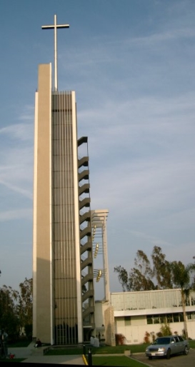
Fluid Viscous Dampers have been installed in many buildings for retrofitting such as the Bennett Federal Office Building in Utah, Christ cathedral tower of hope in Southern California and many more around the world
Fig 1,2 Christ Cathedral Tower of Hope, Orange county, Southern California [7], [8]
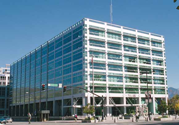
Fig 3 The Bennett Federal Office Building in Salt Lake City, Utah, built in 1965, underwent a major seismic retrofit completed in 2003[9]
2. Types of dampers
Dampers are classified as Tuned mass dampers, friction, shape memory alloys (SMA), viscous, viscoelastic, metal and mass dampers.
2.1Tuned Mass Dampers: –
TMD is a passive damper created in 1970s in United States. It contains movable mass suspended to spring and it’s a frequency dependent device. If we connect TMD to the structure, the seismic energy of structure is transferred to TMD and its energy will be absorbed by the TMD dampers. TMDs have been installed in skyscrapers such, Yokohama Landmark Tower in Yokohama, Aspire Tower in Doha, Citigroup Center in New York City, Shanghai World Financial Center in Shanghai, Trump World Tower in New York City, Burj Al Arab in Dubai, Taipei 101 in Taipei. [10]
2.2 Friction Dampers: –
In this type of dampers, the dissipation of energy is based on the mechanism of solid friction. Friction dampers are most common due to its simple behaviour and easy installation technique. To develop trustworthy friction, the series of steel plates are clamped together with high strength steel bolts. [10]
2.3 Metallic Dampers: –
To dissipate the energy induced to the structure during earthquake, the inelastic deformation of metallic substances was used such as lead and steel for elastic deformation. In conventional structures, dissipation of energy is dependent on the deformation of elastic member. Therefore, it becomes mandatory to replace the dampers when inelastic deformation of the damper occurs for small disturbances. [10]
2.4 Viscoelastic Dampers: –
In the recent years, viscoelastic dampers have been used in major structures to minimize the earthquake effects such as glassy substances or copolymers. Also, because of temperature, the properties of the viscoelastic dampers may vary. Under seismic load, energy is dissipated in a system with & without viscoelastic dampers. [10]
2.5 Shape Memory Alloy (SMA): –
SMA contains special type of material which retains its original shape when subjected to a certain temperature. Due to its properties, Shape Memory Alloy has enormous potential for structural retrofitting and seismic resistance design like, high and low cycle fatigue resistance hysteretic damping, re-centering capabilities energy dissipation capabilities, large elastic strain capacity and excellent corrosion resistance property. In addition to these properties, alloy of nickel and titanium has good resistance to corrosion. [10]
2.6 X Plate Dampers or Elasto Plastic Damper: –
The Elastoplastic dampers are composed of thin metallic plates of one plate or group of plates & available in X and V shape. Mild steel or copper material with varying thickness is used for the preparation of plates. To minimise the vibration on the superstructure due to earthquake, dampers are attached to the superstructure of the building and the foundation. Also, X plate dampers are more effective in dissipation of energy when subjected to seismic vibration. [10]
2.7 Viscous Dampers: –
In recent years, fluid viscous dampers have been used in major civil engineering structures to minimise the effect of earthquakes. The basic principle is that the energy is dissipated through orifice by forcing a fluid which causes pressure difference and thereby force. FVD can be divided in two types: Linear Fluid Viscous Dampers and Nonlinear Fluid Viscous Dampers. In Linear FVD the force is directly proportional to the relative velocity between the ends of damper. When the velocity of the applications is high, nonlinear FVD are used to limit the force capacity of device. FVD has been used due to its easy installation, coordination with other members, diversity in sizes & adaptability. It can be connected in three ways such as damper installed in diagonal braces, damper installed in the foundation or floor & braces and connected dampers in stern pericardial braces. The diagonal and chevron damper–brace systems are two commonly used damper-brace system [10]
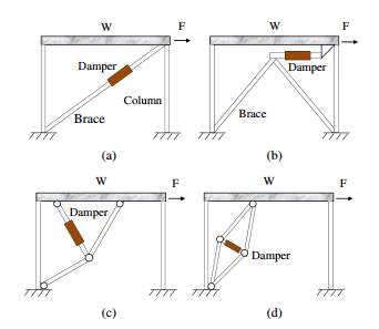
Fig 4 Illustration of a single-story structure with fluid viscous dampers: (a) diagonal; (b) chevron; (c) toggle; (d) scissor [5]
3. Mechanical Model for Fluid Viscous Dampers: –
To describe the dynamic behaviour of FVD two rheological models i.e. the Kelvin-Voigt model and the Maxwell models. Generally, identification of the system could be modelled by physical laws which further reflects the dynamic of a system. This model is called a white box model. However, to create white box in real life is a puzzling task.
To predict the real structural response in structure, it is very important to select proper model for FVD. Generally, Fluid viscous dampers require a model which is made of a set of springs and dashpots connected to each other.
3.1 Kelvin-Voigt model [2]
Many experimental studies showed that the resistance force of some fluid viscous dampers depend on damper deformation and not only on damper velocity.
3.1.1 Linear Viscous Model
The standard linear viscous models are the simplest way to model a velocity-dependent mechanical law. The equation of motion of FVD subjected to time dependent force p is

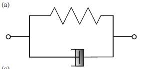
Fig 5 Kelvin–Voigt
This model is extremely simple but sometimes poor for mechanical behaviour representation. Hence, it was updated but the nonlinear viscous models which depends on a fractional exponent of the velocity rather than simple linear relationship.
3.1.2 Generalized Viscous Model
The law of this model has two parameters which was proposed by Constantinou [2]


Fig 6 generalized Kelvin–Voigt
where α is the damping term exponent, whose value lies between 0 and 1. Different values of α are associated withvarious mechanical behaviour. For instance, if α = 1, the linear viscous damping law corresponds; if α = 0, the dry friction appears Due to its ability in modelling of structural behaviours, it has been widely used by various researchers.
However, many experimental studies showed that the resistance force of some fluid viscous dampers depend on damper deformation and not only on damper velocity. The mathematical modelling of this mechanical property can be done by connecting spring element and a viscous element. For instance, if simple linear dashpot relates to linear spring in parallel, the basic Kelvin-Voigt models is obtained. While connecting nonlinear springs with generalized nonlinear viscous models, different behaviours are obtained. Terenzi [2] investigated linear and parabolic models for the elastic force be:
ψe = k1 y (3)
ψe = k2 y2 + k1 y + k0 (4)
where K1 is the elastic stiffness, and K2 and K0 are two constants.
3.1.3 Generalized viscous: linear elastic model
By combining Eqs. (2) and (3), the equation of motion of a generalized Kelvin–Voigt model subjected to a time-dependent force p is derived:

3.1.4 Generalized viscous: quadratic elastic model
In this model, the parabolic form in Eq. (4) is considered without the constant K0:

3.2 Maxwell Model [4]
In this model, dashpot element and spring are connected in series. This model should satisfy kinematic and force conditions.
 (7)
(7)
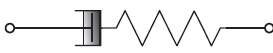
Fig 7 Maxwell model
And force condition
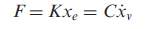 (8)
(8)
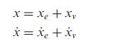
In equation (8), F represents the damper axial force, x denotes the total damper deformation, and xe and xv indicates the deformations of the stiffness and viscous components, respectively. In addition, ẋ, xe, and xv denote the deformation rates corresponding to ẋ, xe, and xv, K stands for the stiffness value of the spring element, and C is the damping coefficient of the viscous element.
Also, by inducing nonlinearity in spring and the viscous element, classical model can be generalized. In generalized model, the resistant forces of both element have fractional exponential coefficients.
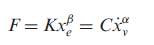 (9)
(9)
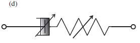
Fig 8 generalized Maxwell model
To simulate a nonlinear FVD, the classical and generalized Maxwell models given in equations (8) and (9) can be used. For these models, two characteristic parameters, K and C for classical Maxwell model, or four characteristic parameters, K, C, α and β for generalized Maxwell model, must be determined.
4. Non-classical Methods in Structural Identification
In past, many diverse types of methods were developed for structural identification. Among them, two evolutive algorithms namely Differential Evolution Algorithm (DEA) and the Particle Swarm optimization (PSO) were investigated due to its stability and simplicity.
4.1 Differential Evolution Algorithms [2]
To solve global optimization problem DEA is simple and powerful population-based stochastic search technique characterized by effectiveness, robustness and simplicity. The basic principle is to construct mutant vector at each generation, for every element of the population. To get target vector, DEA uses
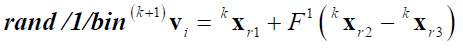
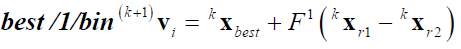
difference of two randomly selected individual vectors. Let consider kxi = {kxi1…,kxij,…,kxin} the ith individual (for i = 1,…,N) at iteration k. The initial population 0xi for i = 1…, N is defined by generating pseudo-randomly the collection of N solutions within the specified search space. At iteration k+1, for each individual kxi a mutation vector (k+1)vi is calculated by one of the following alternative.
 (9)
(9) (10)
(10)  (11)
(11)  (12)
(12)  (13)
(13)
[From Eq. 9 to Eq. 13] r1, r2, r3 and r4 represents randomly selected integers within the set {1,…,i-1,i+1,…,N} and r1 ≠ r2 ≠ r3 ≠ r4. In the population, kxbest is the best performer at the iteration k. The coefficients F1 and F2 are mutation coefficients and also called real positive constants.
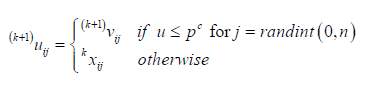
The perturbed individual (k+1) vi and the current population kxiare subjected to crossover operation. The crossover follows the mutation phase and for each mutated vector (k+1)vi a trial vector (k+1)ui (offspring) is created by using the binomial crossover formalized as follows:
 (14)
(14)
In the above equation, pseudo-random number is denoted by u & obtained by using the uniform probability density functions with a range of [0,1]. The parameter pc is the probability of crossover and it ranges between [0,1] and the value is selected by the user. Moreover, radiant (0,n) is a pseudo-randomly integer selected within the set {1,…,j,…,n}.Also, to ensure that at least one parameter is taken into account for constructing the vector (k+1)ui, additional condition is introduced. In case of unconstrained problems, selection operator employs a very simple one-to-one competition scheme between (k+1)ui and (k+1)xi as follows:
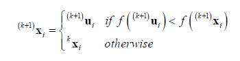 (15)
(15)
Therefore, one must select the best performer from parent individual and its trail one.
4.2 Particle Swarm Optimization (PSO) [2]
PSO is a population-based stochastic optimization used for global optimization. Here, position and velocity can be determined simultaneously as the particle swarm optimization algorithm (PSAO) to which is assumed that the Newtonian dynamic regulates the movement of particles.
The ith particle (with i=1,…,N) at iteration k has two elements, namely position kxi={kxi1,…,kxij,…,kxin} & velocity kvi={kvi1,…, kvij,…,kvin}. In order to protect swarm cohesion, the velocity kvijis forced to be (in absolute value) less than a maximum velocity vj max with vmax={v1 max,…, vj max,…,vn max}. Typically, it is assumed that vmax=γ(xu – xl)/τ but there isn’t any satisfactory degree of uniformity about γ whose numerical value can change in a large interval (usually its value is 0.50). Within the assigned search space the initial positions 0xi for i=1,…,N are expressed by randomly generating the collection of N solutions Moreover 0vij is generated randomly by using uniform distribution between -vj max and +vj max. At iteration k+1 the position (k+1)xi & the velocity (k+1)vi are evaluated as follows
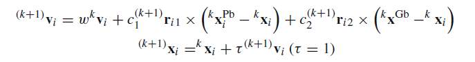 (16)
(16)
Where, w is the inertia weight, c1 and c2 are acceleration factors (called cognitive and social parameter, respectively). In the above equation (k+1)r1i and (k+1)r2i are vectors whose n terms are random numbers uniformly distributed between 0 & 1 and the symbol ‘×’denotes the term-by-term multiplication. The the subscripts on the right side & superscripts on the left side represent different couple of random vectors needed for each particle at all iteration. The symbol kxi Pb denotes the best previous position of the ith particle
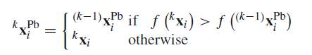 (17)
(17)
Here, 0xi Pb=0xi.
As per the definition of kxGb, information of all particles are shared with each another to know the best performer of the swarm, so that
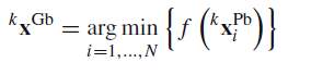 (18)
(18)
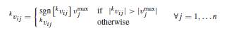
The maximum admissible velocity for each particle I can be checked by performing iteration k in the following manner:
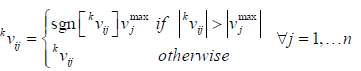 (19)
(19)
5. Literature Review
5.1 Identification of parameters of Maxwell and Kelvin-Voigt generalized models for fluid viscous dampers. [4]
In this publication, author (Rita Greco and Giuseppe Marano,2013) studied Kelvin-Voigt and Maxwell model and commented that this rheological model doesn’t have enough parameters to capture the frequency dependence parameters. So, they decided to develop other models which represent some generalization of basic Kelvin-Voigt and Maxwell models for FVD. Particle swarm optimization(PSO) is adopted to minimize an objective function which represents a measure of difference between experimental and analytical applied forces. They proposed a modification to the classical Kelvin-Voigt and Maxwell models and named them Generalized Kelvin-Voigt model (GKV) and Generalized Maxwell model (GMM). The main difference between the classical and generalized models is that the classical method doesn’t incorporate nonlinearity in both spring and viscous element while generalized model does. Also, to understand the efficiency of generalized models to capture the hysteretic behaviour of Fluid Viscous Dampers, experimental test was performed and verified with analytical model. They recorded the experimental test during dynamic, while analytical results were obtained by applying displacement-time history to mechanical law of candidate. The experiment was tested at SISMALAB laboratory in Taranto, Italy using 750 KN viscous damper. To determine the effective energy dissipation of the device & dynamic performance of the damper, test was performed at different velocities with different cycles. Using non-classical method Particle swarm optimization(PSO) with maximum number of iteration L=100 was applied to a population size N=50. The final identification has been carried out after performing Algorithms 50 times and selecting the best solutions from it. The author compared theoretical and experimental force-displacement and force-velocity for the classical and generalized Voigt and Maxwell model.
From the results, it was clear that the generalized Maxwell model matches with the experimental tests under all test conditions, while Kelvin-Voigt model works less. Voigt model underestimate the force for all test and under low frequency. Moreover, numerical simulation also showed superior results for generalized Maxwell model in stability & capturing real behaviour of FVD considering test condition from which factors have been measured.
5.2 Optimum parameter of a viscous dampers for seismic and wind vibration [6]
In this paper, author Soltani Amir and Hu Jiaxin,2014 studied about the optimal parameters of a passive control device. The basic goal behind this project was to optimize damping ratio of a structure with the help of nonlinear relationship of viscous dampers. When the structure is going back and forth during its oscillation, linear damping has variable energy dissipation. To gain maximum energy dissipation in a system, damping force of nearly uniform and uniform to its possible maximum amount regardless of the position of the structure is the best solution. This system can be designed with parameters to convert the sinusoidal form of the damping force to rectangular form as shown in figure below.
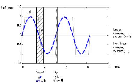
Fig. 9 Maximum damping in non-linear damping system by providing a uniform damping system over a longer time
An optimum damping coefficient can be obtained using nonlinear damping coefficient in a damper as obtained below:
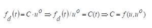 (20)
(20)
Where, C is the optimum damping coefficient, fd(t) is damping force, u is the stroke position in viscous dampers and u° is stroke velocity in the damper
From the above equation (20), it can be said that with time damping coefficient changes and its value will decrease to keep damping force within the criterion where the amount of energy dissipation is
Maximum and the internal force is at minimum level. A MATLAB code was developed to model Single degree of freedom frame which is connected to an active control system and excited by an earthquake record of EL Cento Earthquake-USA 1979.
Finally, they came up with an equation which can be use to make a comparison between the results of the active damping system and the damping system which theoretically governs this equation.
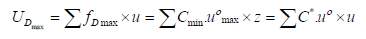 (21)
(21)
They compared the result of linear, non-linear and active damping system considering single degree oscillator and analysed in a time-history analysis program using MATLAB program. 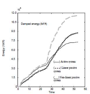
Fig. 10 Damped energy by control systems
From the above figure, we can say that the proposed system shows better performance in controlling the displacement in system response control than the linear system. Also, according to the energy dissipation figure, the loss of energy is greater in non-linear cases compared to the other cases. Finally, we can conclude that the non-linear characterization of the damping system is the only reason for having more energy loss in variable damping case
5.3 Parametric Identification of nonlinear devices for seismic protection using soft computing techniques [1]
In this paper, (Giuseppe Carlo Marano et al, 2013) proposed a new procedure for the dynamic identification of Bouc-Wen parameters of passive devices using evolutionary algorithms and standard laboratory dynamic test. The proposed procedure uses quality control tests & standard pre-qualification to minimize the experimental and mathematical applied force under an imposed displacement-time history. Due to inherent stability and low computation cost, the proposed procedure can be applied to a broad range of mathematical expressions and allows comparison of experimental data & different mechanical laws. From the values of forces obtained, analytical and experimental data are compared to obtain system identification. They recorded the experimental test during dynamic, while analytical results were obtained by applying displacement-time history to mechanical law of candidate. The author used two evolutionary algorithms techniques namely particle swarm optimization and differential evolution to obtain optimal parameters by minimizing the distance between analytical and experimental results. The author decided to identify methods for nonlinear systems based on displacement-force curve only, although they decided to plot velocity-force curve to evaluate the quality of the identification procedure.
The author focused on identifying Bouc-Wen parameters for seismic isolation devices by means of non-classical methods. Particle Swarm Optimization and Differential Evolution are used for parametric identification of seismic isolators. The seismic isolator is modelled without viscous damping as nonlinear single-degree-of-freedom (SDOF) system whose restoring force fBW is:
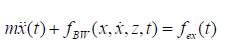 (22)
(22)
where m is the mass, x(t) is the displacement (over dots denote the time-derivative), and g(t) is the excitation dynamic load. Assuming Bouc-Wen hysteresis model, the restoring force is:
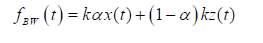 (23)
(23)
where α is the ratio of the post-yield kp to pre-yield k(elastic) stiffness, z(t) is the hysteretic parameter given by the following nonlinear differential equation:
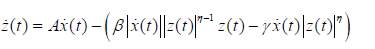 (24)
(24)
where A, β, γ and η are dimensionless quantities controlling the behavior of the model. Parameters β and γ control the shape of hysteretic loops, η controls the sharpness from initial slope to the slope of the asymptote. The Bouc-Wen hysteresis model can be designed fully if the parameters k, α, β, γ, and η are identified.
The testing machine used consist of high resistance steel frame to withstand 10000kN compression in vertical direction and 2200kN horizontal load with maximum allowable horizontal displacement of 260mm. Visualization, Data acquisition and real-time system control was achieved by using LABVIEW. Under three vertical loading conditions (440kN, 840 kN and 1120 kN). For each test, DEA & PSO are performed 100 times to check the stability of the identification procedure. Load-time, load-displacement and load-velocity comparison between experimental data and numerical obtained using different viscous model and DEA. The proposed model is efficient and stable and can be used for the parametric identification of seismic isolators as the procedure only requires reaction forces and time histories of displacement. Also, the result from the analytical and experimental showed good agreement.
5.4 Design method for fluid viscous dampers [11]
In this paper, fluid viscous dampers with double guided bars is presented for basic design method. The flow of the viscoelastic fluid is analyzed between two parallel plates, one of which is still and the other of which is still. The shear stress and the velocity of the fluid at the fringe of piston are solved approximately. Also, a mathematical model is derived for viscous dampers and the shock test is carried out. Based on the fractional damping model, basic design equation is derived. Thus the dimensionless velocity obtained as,
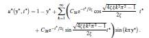 (25)
(25)
The coefficients C1k = −2/kπand C2k = −2/kπ_4ζξk2π2 − 1 in equation 25 can be easily obtained from
Eqs. (26) and (27).
 (26)
(26)  (27)
(27)
When y* and t* are small enough, a simper function is introduced to replace the instantaneous velocity of flow. In this model, damping coefficient C is obtained as
C = Kμπdle−ϑh. (28)
The shock test is carried out using a drop machine to choose the viscosity for the material. A drop hammer with 9.8kg mass is lifted to a certain prescribed height and then falls freely to impact on the piston of the damper. Data acquisition system and an acceleration transducer B&K4393 are used to record the acceleration time history of the drop mass when it falls. The piston of the damper was changed regularly and the length of piston chosen for test were 30mm with diameters of 42,46,48,50 and 52mm respectively. Then the piston with diameter of 46mm were chosen with length 15,18,20,25 and 30mm respectively. From the results of experimental value and the analytical value it is found that the difference is 6.02% which satisfy the specification in GJB150.18. From the shock test, it is clear that the nonlinearity of the damper is mainly dependent on the damping materials and not n the physical dimensions. To meet the requirement of engineering practice, specimen damper was designed using this model. Shock test was performed on this specimen sample which showed that the chosen physical dimension of the dampers is appropriate. The mechanical characteristics of the specimen damper are analysed which showed a decent relation between experimental results and the analytical results, which confirms the mechanical model.
6. A comparative study on parametric identification of fluid viscous dampers with different models [2]
The author (Rita Greco et al,2014) decided to compare parameters of FVD with various existing literature models to identify the proficiency of these models to match experimental loops under different test specimens. The experimental and analytical values of forces are compared with each other to develop the identification process. The results from experiment are recorded during dynamic test while analytical results were obtained by applying time history of displacement to the candidate mechanical law. The experimental data is obtained using different classical and generalised mechanical models which was discussed in section 3. To define the objective function in the identification problem, following integral is assumed:
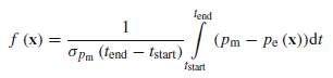 (25)
(25)
Where, tstart and tend are the start and end time records, respectively, pe(t) is the force estimated & pm(t) is the force measured. Equation 25 is obtained by numerical differentiation of experimental displacement
Time history with respect to the third-order algorithm to limit numerical noise.
6.1 Test apparatus
Viscous damper with capacity of 750 kN was tested at SISIMALB srl laboratory in Taranto, Italy. The high-resistance steel frame can withstand a tension and compression loads of 2200kN. The ends of the structure are anchored to the steel frame using pin and a threaded connection. A load cell of 2,500kN is located between the servant cylinder and the device to acquires the forces applied to the device during the entire duration of the experiment. Using computer automatic control hydraulic pressure system to change the applied force, control and data acquisition system can generate a real-time analysis of device displacements. This system can control applied forces in real time with respect to the force imposed test or imposed displacement.
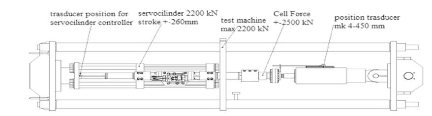
Fig 11 Fluid Viscous Damper and Viscous test machine
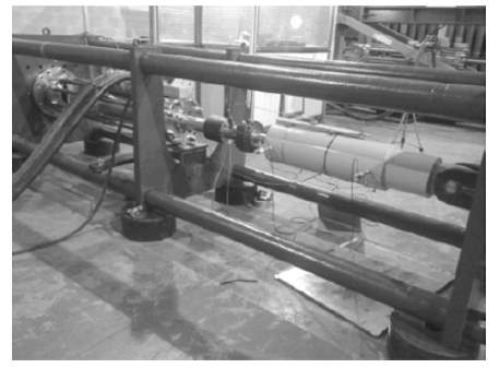
Fig 12 Picture of the test apparatus with the fluid viscous damper

Table 1 Fluid viscous damper design condition
6.2 Test Cases
To obtain dynamic response of the viscous damper, four experiments were performed. The basic objective of the experiment is to evaluate the effective energy dissipation of the device and to determine the dynamic characteristics of the damper at varying velocities. The results were obtained for different velocities with peak velocity of 92, 230, 460 and 460mm/s. The first three tests with 3-cycle excitation period and the fourth test (energy dissipation test) with 10-cycle period
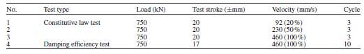
Table 2 Fluid viscous damper test condition
The check on the maximum admissible velocity for each particle i is performed at iteration k using the following equation:
 (26)
(26)
Second check, to verify the feasible search space of particle
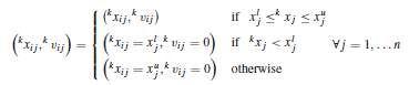 (27)
(27)
In the above equation, unfeasible particle velocity is taken as zero for the next iteration, to avoid any points outside the search space.
6.3 Parametric Identification
The parametric identification using PSO was applied to a population size N = 50 with a maximum number of iterations L = 100 to evaluate the optimal values of the unknown parameters shown in equation (1), (2), (5), (6). To solve the single-objective optimization problem given in equation (25), parametric identification has been performed. The best solution from the fifty solutions using algorithms has been carried out as the final identification result. Objective function results obtained from the PSOA using the linear viscous mechanical model for four different experimental test
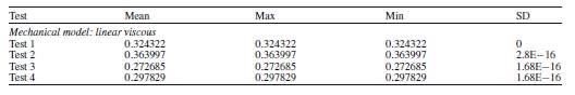
Table 3 Objective function results obtained from the PSOA using the linear viscous mechanical model for four different experimental tests
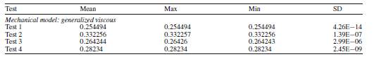
Table 4 Objective function results obtained from the PSOA using the generalized viscous mechanical model for four different experimental tests
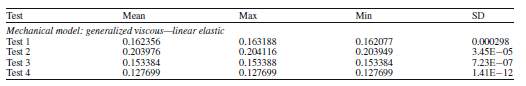
Table 5 Objective function results obtained from the PSOA using the generalized viscous—linear elastic mechanical model for four different experimental tests
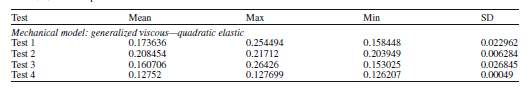
Table 6 Objective function results obtained from the PSOA using the generalized viscous—quadratic elastic mechanical model for four different experimental tests
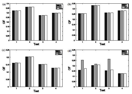
Fig. 13 Histograms of data in Tables 3, 4, 5 and 6: a Linear viscous, b generalized viscous, c generalized viscous—linear elastic, d generalized viscous—quadratic elastic
Now the values obtained from the linear viscous models are used to obtained mechanical parameters for different velocities shown in table 7,8,9 & 10.
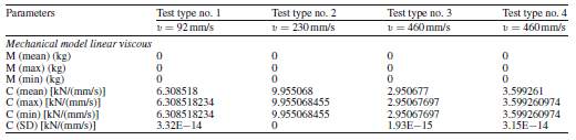
Table 7 Values of mechanical parameters obtained in four different test types, using the linear viscous mechanical model of FVD
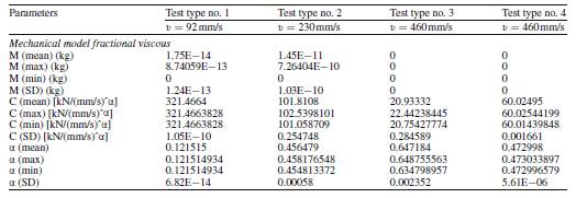
Table 8 Values of mechanical parameters obtained in four different test types, using the fractional viscous mechanical model of FVD
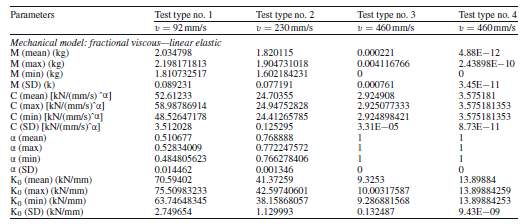
Table 9 Values of mechanical parameters obtained in four different test types, using the fractional viscous—linear elastic mechanical model of FVD
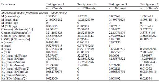
Table 10 Values of mechanical parameters obtained in four different test types, using the fractional viscous—quadratic elastic mechanical model of FVD
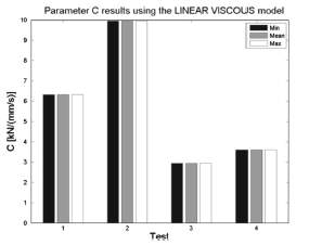
Fig. 14 Histograms of values of mechanical parameters obtained in four different test types, using the linear viscous mechanical model of FVD
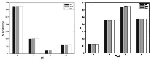
Fig. 15 Histograms of values of mechanical parameters obtained in four different test types, using the fractional viscous mechanical model of FVD
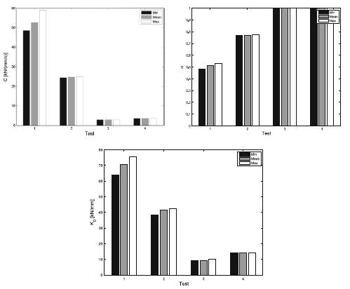
Fig.16 Histograms of values of mechanical parameters obtained in four different test types, using the fractional viscous—linear elastic mechanical model of FVD
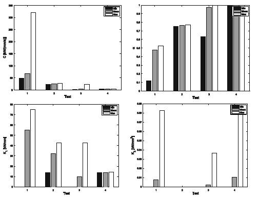
Fig.17 Histograms of values of mechanical parameters obtained in four different test types, using the fractional viscous—quadratic elastic mechanical model of FVD
6.4 Comparison of hysteresis loops predicted by various models
The simulated models which was discussed previously are compared with the experimental hysteresis loop of the damper under investigation for velocities V1, V2, V3 and V4. In the fig 18 & 19, relation between force and displacement and in the fig 20 & 21, relation between velocity and force are shown. Also, the solid lines show the theoretical loops, while the dotted lines indicate the experimental loops.
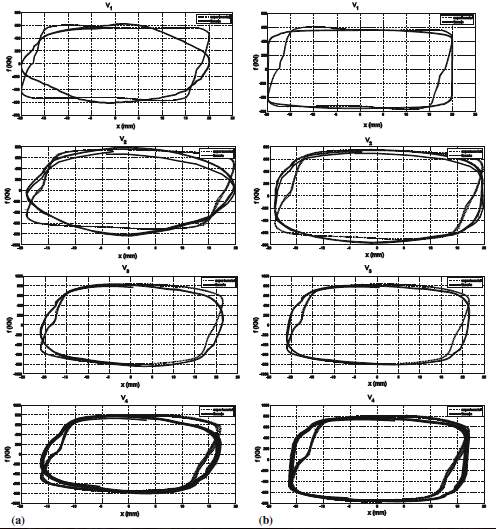
Fig.18 Comparison between theoretical and experimental force–displacement relationship: a Linear viscous model, b generalised viscous model. Continuous line theoretical dashed line experimental
From the plots, we can say that the theoretical loops and experimental loops have relatively same velocity and displacement. Also, the above figures show that the hysteric loop varies with an increase in velocity. The result of the theoretical and experimental loops obtained from generalised viscous—linear elastic model shows (fig) that under all frequencies matches well. Also, for linear viscous elastic models,the experimental loops is better. On the other hand, other models showed elliptical hysteresis loops. Therefore, these experimental loops are not a good match under all frequencies due to varying shape from low to high frequencies.
Comparing generalised viscous—linear elastic [(c) in Fig. 9] with generalised viscous—quadratic
elastic [(d) in Fig. 9] showed a good match with experimental loops for all velocities. In spite of predicting well force by third and the fourth model, one must consider the area of the loop, which shows the amount of energy dissipated in one cycle. From the plot of generalised viscous—linear elastic we can say that the model overestimates the amount of energy dissipated for all velocities while, generalised viscous—quadratic elastic predicts well the dissipated energy for all velocities. generalised viscous—quadratic elastic model shows the same observations as generalised viscous—quadratic elastic
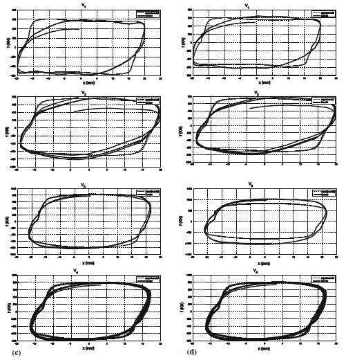
Fig.19 Comparison between theoretical and experimental force– displacement relationship: c Generalised viscous—linear elastic, d Generalised viscous—quadratic elastic. Continuous line theoretical dashed line experimental
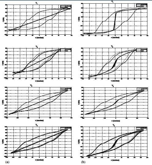
Fig.20 Comparison between theoretical and experimental force– velocity relationship: a Linear viscous model, b generalised viscous model. Continuous line theoretical dashed line experimental
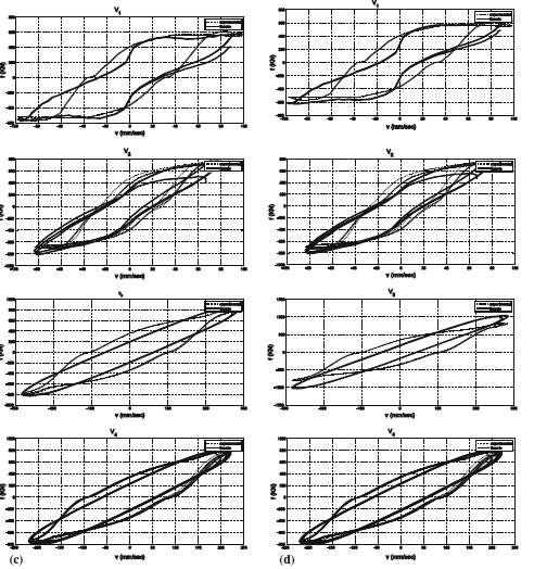
Fig.21 Comparison between theoretical and experimental force– velocity relationship: c Generalised viscous—linear elastic, d generalised viscous—quadratic elastic. Continuous line theoretical dashed line experimental
Fig 20 and 21 shows the relationships between velocity and force. The first two models do not predict well the experimental force-velocity loop, while the other two does shows satisfactory experimental loops, especially under high excitation of frequency.
We know that the matching of experimental model depends on the excitation frequency. So, it will be interesting of we know the sensitivity of identified parameters for all frequency excitation. Therefore, the mean value p for each p is evaluated from each test and extrapolated, the range of variation ∆p =pmax – pmin and the ratio ∆p/p are equipped in the above table to understand the variability of parameters with respect to the test conditions. From the above tables, one can say that except for the linear viscous model, the parameter C shows inconsistency against the velocity of the external excitation application. In general, all model which has been analysed showed comparable variability of involved parameters.
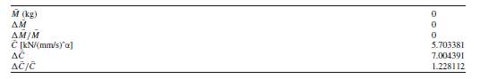
Table 11 Parameters sensitivity of linear viscous mechanical model
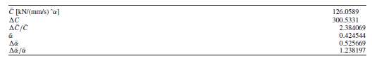
Table 12 Parameters sensitivity of generalised viscous mechanical model
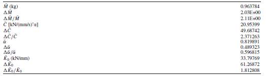
Table 13 Parameters sensitivity of generalised viscous—linear elastic mechanical model
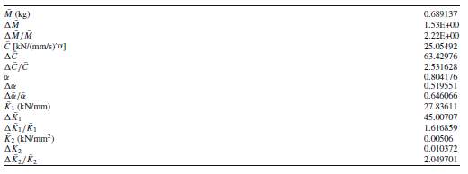
Table 14 Parameters sensitivity of generalised viscous—quadratic elastic mechanical model
7.Conclusion
This study has been conducted on classical and generalised mechanical model for FVD. The experimental and analytical values are compared to identify the forces experienced by the device under investigation. In total, four experiments have been performed to understand the dynamic response for FVD. When comparing the results of generalised viscous-linear model obtained from the experimental loops to the analytical loops, under all excitation frequencies, showed good match, while linear viscous elastic one showed better result. The generalised viscous-linear elastic and generalised viscous-quadratic elastic showed good match with experimental loops for all velocities of the load application. Moreover, the generalised viscous-linear elastic overestimates the amount of energy dissipation under all velocities. while, generalised viscous-quadratic elastic estimated well the energy dissipated, especially under high-velocity load application. Also, the sensitivity of the identified parameters has been investigated against the frequency excitation. From the results, one can say that except for the linear viscous model, the parameter C shows inconsistency against the velocity of the external excitation application. In general, all model which has been analysed showed comparable variability of involved parameters.
The results obtained here were purely based on the parametric identification techniques. So, author must consider nonparametric identification techniques as this technique is more suitable in structural health monitoring, due to change in system characteristic over time, both quantitatively as well as qualitatively. Also, it is needed to compare both parametric and nonparametric using real data carried out from nonlinear viscous dampers of full scale.
8. References
1) Giuseppe Carlo Marano, Rita Greco, Giuseppe Quaranta, Alessandra Fiore, Jennifer Avakian and Davide Cascella: Parametric identification of nonlinear devices for seismic protection using soft computing techniques, Advanced Materials Research Vols. 639-640 (2013) pp 118-129
2) Rita Greco, Jennifer Avakian, Giuseppe Carlo Marano: A comparative study on parameter identification of fluid viscous dampers with different models Arch Appl Mech (2014) 84:1117–1134
DOI 10.1007/s00419-014-0869-3
3) Iztok Fister, Amir H. Gandomi, Iztok Jr. Fister, Mehdi Mousavi, Ali Farhadi : Soft Computing in Earthquake Engineering: a Short Overview ,International Journal of Earthquake Engineering and Hazard Mitigation (IREHM), Vol. 2, N. 2 ISSN 2282-7226 June 2014.
4) Rita Greco1 and Giuseppe C Marano2: Identification of parameters of Maxwell and Kelvin–Voigt generalized models for fluid viscous dampers, Journal of Vibration and Control 2015, Vol. 21(2) 260–274
5) Tong Guo, MASCE; Jia Xu; Weijie Xu; and Zhiqiang Di: Seismic Upgrade of Existing Buildings with Fluid Viscous Dampers: Design Methodologies and Case Study, DOI: 10.1061/(ASCE)CF.1943-5509.0000671
6) Soltani Amir, Hu Jiaxin: Optimum Parameter of a Viscous Damper for Seismic and Wind Vibration, International Journal of Civil, Environmental, Structural, Construction and Architectural Engineering Vol:8, No:2, 2014
7) https://structurae.net/structures/tower-of-hope
8) http://occatholic.com/tower-of-hope-earns-award-of-excellence/
9) https://pubs.usgs.gov/fs/2005/3052/
10) Alireza Heysami: Types of dampers and their seismic performance during an earthquake, Current world environment Vol, 10(special issue 1), 1002-1015(2015)
11) Jia Jiuhong · Du Jianye · Wang yu · Hua Hongxing: Design method for fluid viscous dampers, Arch Appl Mech (2008) 78: 737–746
Cite This Work
To export a reference to this article please select a referencing stye below:
Related Services
View all


Related Content
All TagsContent relating to: "Computing"
Computing is a term that describes the use of computers to process information. Key aspects of Computing are hardware, software, and processing through algorithms.
Related Articles

DMCA / Removal Request
If you are the original writer of this dissertation and no longer wish to have your work published on the UKDiss.com website then please: