Dissertation on Hydrological Models

COMPARISON BETWEEN TWO MODELS: THE CASE OF THE UPPER BLUE NILE BASIN

Introduction

Water is the source of life on Earth. Sustainable use and management of water resources are important for a healthy existence of humans and different ecosystems. Hydrological modeling is an important tool that is being used to assist the proper water management. There are different hydrologic models that were developed and used around the world for different purposes. These models are different in their structure, methods, and the data they require. There are many classifications to these models. One of them is according to the extent of physical principals represented in the model: physical, empirical, and conceptual models. Models also can be classified based on the variation of their parameter values in space and time into lumped, distributed, and semi-distributed models. There is continues debate about which model is better to use. Some argue that physically based model reflects better the nature of different processes. Others see that physical models are computationally expensive, and still do not reflect the heterogeneity of catchment properties. Also, hold more uncertainty as more parameters are usually required. Some consider conceptual models to be more reliable due to less computation time, high efficiency to simulate flows, and wide applicability.

In the light of the previous discussion, the objective of this study is to compare between two models that are different in terms of physics and discretization. This comparison is based on their ability to generate the observed flows at the basin outlet. Attempting to answer the big question of which model is better to use. The remainder of this document is organized as: section 2 is a description of the study area, section 3 is the methods used, section 4 includes the results and discussion, and section 5 is the conclusions made.

Description of Study Area

The Upper Blue Nile Basin (UBNB) is located in the North-Western part of Ethiopia and its outlet as Figure 1a shows is at the location of the Grand Renaissance Ethiopian Dam (GERD). The basin has a drainage area of 176,000 km2. Most of this area is a part of the Ethiopian plateau which has high elevations exceeds 4200 meters. While the western part of the basin as Figure 1b shows has relatively low elevations that reach 495 meters at the basin outlet near the Sudanese borders. The climate of the basin is tropical highland monsoonal with the major part of the rainfall falls between June and October (Conway, 1997). The basin average rainfall is 1600 mm/year and varies spatially from 1000 mm/year near the outlet to 1800 mm/year at the eastern plateau (Sutcliffe & Parks, 1999). Annual potential evapotranspiration is estimated to be about 1100 mm/year (Kim et al., 2008). The average annual outflow of the basin is in the order of 1500 m3/sec and 80% of the water volume flows during the rainy season(Conway, 1997). The basin runoff ratio is around 17% which reflects the high losses possibly due to evapotranspiration, interceptions, and ground water recharge. The high significance of the basin comes from its high contribution to the Nile, in which the basin contributes 50% – 60% of the flow that reaches Egypt. Most of the published studies about the Nile was in this area because of its high importance and data availability (Betrie et al.,2011; Liu et al.,2008; Rientjes et al., 2011; Woldesenbet et al., 2017).

 

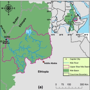
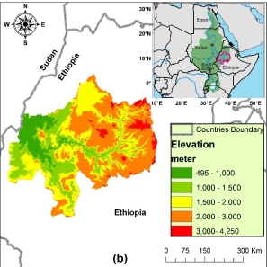
Figure 1.  Map showing (a) Location of Upper Blue Nile Basin, and (b) Elevation (SRTM- 90 m).

Methods

Two different models reflecting different degrees of complexity, structure, and discretization were applied to a study area and were compared and evaluated based on their accuracy in simulating observed flows. One is the HBV (Lindström et al., 1997) that is a simple conceptual model, and SWAT that is a complex model (Neitsch et al., 2005). Evaluation criteria includes: (I) model performance in calibration and validation at daily time steps: The model is calibrated using Dynamically Dimensioned Search (DDS; Tolson & Shoemaker, 2007) and Pareto Archived Dynamically Dimensioned Search (PA-DDS; Asadzadeh & Tolson, 2009) and its performance is evaluated using the Nash Sutcliffe efficiency (NSE) coefficient and Nash-Sutcliffe efficiency with logarithmic values (Log(NSE)).  (II) The ability of the model to capture the variability or seasonality in flow pattern: the resulted flow series of PA-DDS is used and separated to low and high flows then evaluated based on NSE.  (III) Model performance evaluation at multiple time-scales: Model outputs and observed flows were compared using NSE at aggregated time scales to assess if the same model can be used to obtain streamflows of different timescales.

3.1 Description of Models

HBV is a simple conceptual model that has been applied in a large number of studies worldwide (Bergstrom, 2014). The model was originally developed at the Swedish Meteorological and Hydrological Institute (SMHI) in the 1970s. The version used in this study is HBV-96 (Lindström et al., 1997), which is the revised version by the Swedish Association of River Regulation Enterprises (VASO) and SMHI. Figure 2a shows the structure and processes used by HBV to generate the streamflow. The model simulates the different processes by using connected buckets (reservoirs) that are governed by empirical equations. The model consists of 4 buckets that are used to simulate daily flow, the first one is for the snowmelt and accumulation processes. The second is representing the unsaturated soil processes taking in rainfall and snowmelt. The output of the second bucket is divided between two more buckets, one is a non-linear bucket (Fast reservoir) that represents the fast processes in a basin, which are the direct runoff and lateral flow summed together. While the second one is a linear bucket (Slow reservoir) that represents the slow basin response, which is base flow. The output of fast and slow reservoir is summed to get the final sub-basin flow. A routing routine is used to route this flow in the main stream up to the outlet of the basin.

SWAT is considered a complex physically-based model that can run on GIS interface at daily time step and can be used to simulate flows, sediment, and agriculture yields from large watersheds with spatially varied soil, land cover and management practices over a certain period of time(Neitsch et al., 2005). The model as shown in Figure 2b includes many processes and allows for a part of the precipitation to be intercepted by plants (canopy storage), and the remaining part to infiltrate the soil or to flow as surface runoff. The surface runoff can be provided with a lag-time to represent large basins with high times of concentration. The infiltrated water is divided between soil moisture, lateral flow, and ground water. The ground water in SWAT is divided to two reservoirs one is shallow aquifer that contributes  to the main stream as base flow and a deep aquifer that contributes no flow to the main stream and water stored in this reservoir is considered as losses out of the system( Arnold et al., 1993). SWAT also allows for routing of ground water to move horizontally and vertically. The summation of surface runoff, lateral flow, and base flow is then the total flow that is routed through the main stream, where also transmission losses can be calculated.

SWAT is considered more complex compared to the HBV. In addition to the model structure discussed above, SWAT is more complex regarding other two aspects: discretization and parameters, and required data. In terms of discretization and parameters, both SWAT and HBV also allow for discretization of the basin. However, SWAT has the ability to handle finer discretization defined as Hydrologic Response Units (HRU) which are areas of homogeneous characteristics for soil, land cover, management practices, and slopes (Arnold et al., 1998). However, HBV can only be discretized up to sub-basins and does not allow for further discretization. Definition of parameters also varies between HBV and SWAT. HBV has only 8 parameters and SWAT has 15 parameters. Table 1 shows the parameters considered by both these models.

In terms of data requirement, SWAT and HBV use different equations to model the hydrological processes and hence, their data requirement vary. The data requirement for SWAT is higher than that of HBV as it handles calculation at finer resolutions (in terms of discretization). Data include soil data, land cover data, and digital elevation data in order to extract the properties of each HRU. However, HBV is a simple conceptual model that does not require information on land cover and soil and can be provided with only meteorological data like daily rainfall and temperature. Overall, it can be concluded that SWAT is more complex and requires more computation effort and time compared to HBV.

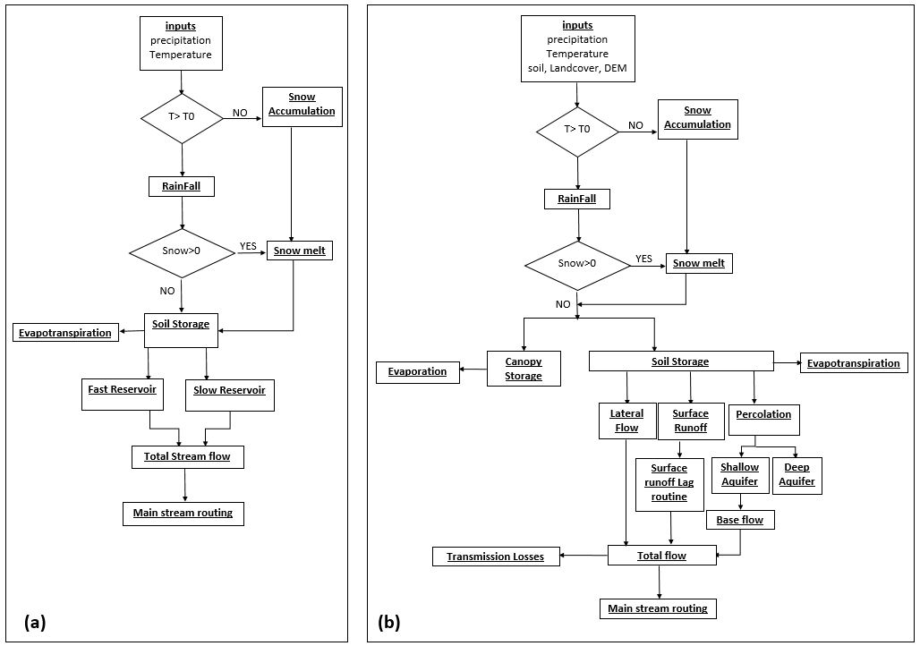
Figure 2. Structure and General Processes in (a) HBV, and (b) SWAT.

Table 1. Model parameters and their calibration range for HBV and SWAT.

HBV
Parameter	Discerption	Calibration Range
ETF	temperature anomaly correction factor	0-1
LP	Limit for PET-soil moisture content below which evaporation becomes supply-limited	0-1
FC	Field Capacity (mm)	50-1500
beta	Soil release parameter	1-3
FRAC	fraction of soil release that goes to fast reservoir	0.3-0.7
K1	Fast reservoir coefficient	0.1-1
alpha	fast reservoir exponent	1-3
K2	Slow reservoir coefficient	0-0.1
SWAT
Parameter	Discerption	Calibration Range
RCHRG_DPa	Deep aquifer percolation fraction	0-1
GWQMNa	Threshold water depth in shallow aquifer required for base flow to occur (mm)	0-5000
GW_REVAPa	Ground water moved by capillarity to upper layers “revap” coefficient	0.02-0.2
CANMXa	Maximum canopy storage	0-10
GW_Delaya	Delay time for aquifer recharge (days)	15-450
REVAPMNa	Threshold depth of water in the shallow aquifer for “revap” to occur (mm)	0-500
CH_K2a	Channel effective hydraulic conductivity	0-75
ALPHA_BFa	Base flow recession factor	0-1
CH_N(2) a	Manning’s “n” value for the main channel	0-0.3
SURLAGa	Surface runoff lag time (hrs)	0-24
SOL_Z()b	Soil Layer depth	-0.5-0.5
CN2 b	SCS-Curve number	-0.25-0.25
SOL_AWC()b	Available water capacity of soil layer (fraction of water volume)	-0.5-0.5
SOL_K()b	Soil layer Saturated hydraulic conductivity (mm/hr)	-0.5-0.5
SLSUBBSN b	Average slope length (m)	-0.25-0.25

a: Parameter is changed by replacing its value by single value in all HRUs in calibration, validation, and sensitivity analysis.

b: Parameter is changed by multiplying (1+ value) in calibration, validation, and sensitivity analysis.

Data and Model Setup

Data Description

For both SWAT and HBV meteorological data is essential. The meteorological data available is a group of 6 observation stations (see Figure 3a) that have daily rainfall and temperature time series covering the period of (1987-1998). These stations are not covering the whole basin as Figure 3a shows, thus another source of forcing data was used to cover the area that missing observations downstream of the basin. This other source of data used is the gridded data set of Climate Forecast System Reanalysis (CFSR; Dile & Srinivasan, 2014; Fuka et al., 2013) daily time series for rainfall and temperature. To check the consistency of using this data along with observations, three stations at different locations were compared based on the number of rainy days and total monthly volumes. The results of the comparison (not shown here for space limits) showed minor errors of less than 10%. Further, two trial runs were carried out, one by using the combination of two sources data, and another trial with only the 6 observation stations. The model was calibrated in each of the two trial runs and the results were improved by using the mixed data sources, which give confidence in using the mixed sources as a solution to the data availability problem. The flow time series is another type of data that is needed by HBV and SWAT to calibrate the two models. Observation gauge data available is at ELDeim station which is located at the outlet of the basin (see Figure 3a), the data is daily time steps and covering the period of (1965-2014).

Different from HBV, SWAT requires topographic, soil, and land cover data to characterize the different HRUs. For topographic data, SRTM-90m digital elevation map is used(Lehner et al., 2006). Figure 1b shows this data, it can be noticed that elevations vary in a relatively wide range. Values are around 495m at the outlet and exceed 4200m at the eastern part of the basin. The land cover data used in SWAT model is GLOBCOVER 2009 v2.3 (Bontemps et al., 2011). Figure 3b shows the spatial distribution of the different land cover classes. The major land cover classes in the basin are agriculture, shrubs, forests, and grassland. The source of soil data used in SWAT is the International Soil Resource and Information Centre (ISRIC) that has compiled a draft 1:1 million scale soil map for North East Africa(van Engelen & Dijkshoorn, 2013). For each of the horizontal layers, FAO soil classification depth of layer, texture and other physicochemical properties are provided. The data analysis showed that the dominant soil types are 19 % of Latosol and Alisols, 18 % of Nitosols, 17% of Vertisols, and 10% of Cambisols.

Model Setup

The basin is discretized to 9 sub-basins (see Figure 3a) using the delineation tools in GIS. SWAT further uses the classes of soil, land cover, and slopes to form different combinations and build the HRUs. For the study area, 484 HRUs were built. The aim of this fine discretization in SWAT is to maintain the spatial variability of basin characteristics. Thus, Some of the model parameters are varied spatially from one HRU to another, these are the last 5 parameters listed in Table 1 (i.e. SOL_Z(), CN2, SOL_AWC(), SOL_K(), and SLSUBBSN).while for the other parameter they are fixed spatially. The direct runoff in SWAT can be modeled using either the soil conservation service (SCS) curve number (CN) method (USDA, 1972) or the Green–Ampt infiltration method(Green & Ampt, 1911). For this study, the (SCS) curve number (CN) method was used because it can use daily input data (Neitsch et al., 2005; Arnold et al., 1998). SWAT can calculate the potential evapotranspiration using three different methods: Priestly–Taylor(Priestley & Taylor, 1972), Penman–Monteith (Monteith, 1965), and Hargreaves (Hargreaves et al., 1985). For this study, Hargreaves method was used because it requires only temperature and hence suits the limited climate data available in the study area. (Arnold et al., 1993). In SWAT the daily water volumes are calculated for each HRU and summed up at the sub-basin outlets then routed through the river network to the basin outlet. The river routing can be done using two methods: variable storage or Muskingum routing methods. For this study, the Muskingum method was used to route flows.

For HBV, the model is discretized into 9 sub-basins the same way as for SWAT (see Figure 3a). the discretization was made to maintain the spatial variability of meteorological data while parameters are assumed to be the same all-over the basin for simplicity. HBV also requires the areas of the delineated sub-watersheds; these areas were extracted from GIS and provided to the model. in addition to the daily rainfall and temperature data, HBV requires the monthly average potential evapotranspiration as input data to estimate the actual evapotranspiration. The daily potential evapotranspiration was calculated using Hargreaves method the same as in SWAT then the average monthly is calculated and incorporated to the model input data. The model calculates the daily flow volumes at the outlet of each sub-basin, then flows are routed through the main stream to the final outlet of the basin using Muskingum method.

The two models were set to run in the same period as the meteorological data (i.e. 1987-1998). The first two years are used as a spin up period and the reaming is divided between calibration (1989-1993) and validation (1994-1998).  To calibrate the models, a MATLAB code was written and used to couple SWAT with the calibration algorithms used in this study (i.e. DDS and PA-DDS). While for HBV, the version used here was already coded in MATLAB and coupled with the same calibration methods.

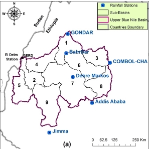
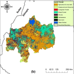
Figure 3. Map showing (a) UBNB Discretization and Rainfall Stations and (b) Spatial distribution of land cover classes (GLOBCOVER 2009 v2.3).

Calibration Methods

The DDS is a stochastic simple heuristic global search algorithm that can be used for the calibration of hydrological models. It starts the search globally and as the algorithm precedes the search becomes more local by reducing the number of parameters probabilistically in the neighborhood. The algorithm goes through a number of function evaluations that is specified by the user. At each time the function is evaluated the current solution is compared with the best-archived solution (candidate solution) if the current solution is better it replaces the archived one. To create the new candidate solution, the current solution values are perturbed for the randomly selected parameters only. The magnitude of this perturbation is randomly selected from a normal distribution with the mean of zero(Tolson & Shoemaker, 2007).

One of the main limitations of DDS is that it is a single-solution based approach that focuses on modifying and improving a single candidate solution, which implies that the algorithm is more likely to find a local optimum solution. To overcome this problem the algorithm might be repeated for serval iterations with different randomly selected start locations (initial parameter values). So, for this study DDS calibration is carried out for 10 iterations. For each iteration, the number of function evaluations was set to 1000, because Tolson & Shoemaker (2007) showed that 1000 function evaluations are enough to reach stable results for DDS with SWAT model. Two cases are carried with DDS, first case objective function is set to Nash Sutcliffe model efficiency coefficient (NSE) , and second case Nash-Sutcliffe efficiency with logarithmic values (Log(NSE)).

In addition to DDS the calibration of the two models was also made using a multi-objective technique. The  PA-DDS method is used with two metrics for objective functions: NSE and Log(NSE). The PA-DDS is built on the same algorithm of DDS but the output is what is called Pareto-front (trade-offs)which is a group of sets of objective function values that are not-dominated with any other solution. Rather than perturbing one solution as in DDS, the PA-DDS perturbs the group of points in the Pareto-front until it reaches to the best (non-dominated) Pareto-front. For this study, one iteration with 10,000 function evaluations was carried out.

Results and Discussion

Calibration and Validation

The results of 10 different iterations of DDS calibration method using NSE as objective function showed very good results of NSE ranging from 82% to 92% for SWAT and from 88% to 91% for HBV during calibration period, and 75% to 85% and 72% to 83% for SWAT and HBV during validation period, respectively. Figure 4 shows hydrographs for the best solution (i.e. highest NSE) out of the 10 trials. Results indicate the capability of HBV to produce flows comparable to a more complex model like SWAT. Three main observations were made while calibrating the two models.

First, the two best solutions of HBV and SWAT shown in Figure 4 indicate underestimation of the peaks for most of the years. However, further scrutiny of the hydrographs simulated by the remaining 9 iterations indicated that there are other solutions that match the observed peaks in magnitude but have a marginally low NSE value compared to the best solution. This reflects the importance of using visual inspection in parallel to using a metric that captures the overall accuracy of the model when choosing a calibrated set of parameter.

Secondly, by analyzing the10 iteration results it was found that 5 of them have NSE values in a very close range between 90%-92%, but the range of optimal parameters was wide. However, the parameter range was observed to be wide indicating that multiple parameter sets could be used to arrive at the best solution, also known as “equifinality” principle (Beven & Freer, 2001). Thus, without the knowledge of real parameter values (or range), it will be difficult to know which set is representing reality especially for conceptual models that have less physical and measurable parameters.

Thirdly, some of the iterations showed good solutions in terms of simulated flows, however when the state variables (i.e. soil storage or moisture, and bucket storages) were found to exhibit an accumulating behavior (i.e. the storage is increasing monotonically) which is not realistic. This monotonic increase might reflect the deficiency in the model structure and parameterization, especially for HBV as the model does not allow for losses, and the increasing storage in the system is due to the model attempting to accommodate the large deficit between rainfall and outflow.

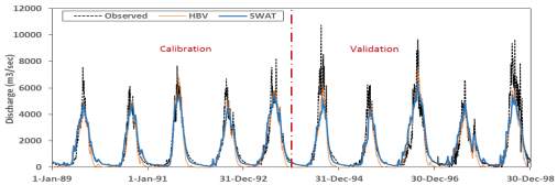
Figure 4. Hydrographs of best solution for HBV and SWAT using DDS method with NSE as objective function metric.

To reduce the effect of any systematic under-or-over estimation of low flows as shown in Figure 4, DDS calibration is repeated by replacing the NSE with Log(NSE) as the objective function. The results of 10 different iterations show very good results of Log(NSE) ranging from 89% to 94% for SWAT and 91% to 92% for HBV during the calibration period and 85% to 91% and 82% to 85% for SWAT and HBV respectively during the validation period. Figure 5 shows the hydrograph corresponding to the best solution (i.e. highest Log(NSE)) where it can be observed that both models are performing well in calibration (Log(NSE) equal to 92% and 94% for HBV and SWAT respectively) and validation (Log(NSE) equal to 85% and 91% for HBV and SWAT respectively). The ability of SWAT to perform better can be attributed to the differences in the model structure, as SWAT simulates the ground water and base flow in more detailed way by considering the lag between different layers and between aquifers, which is more realistic compared to the lumped linear bucket used to model the base flow in HBV.

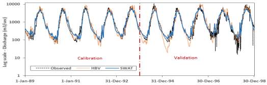
Figure 5.  Hydrographs of the best solution for HBV and SWAT using DDS method with Log(NSE) as objective function metric (Hydrographs are plotted on log-scale).

Calibration was also carried out in a multi-objective framework with two objective functions, NSE and log(NSE) using the PA-DDS algorithm. A total of 10000 model evaluations were carried out and the results of non-dominant solutions are shown in Figure 6. It can be observed from the figure that SWAT is able to perform better than HBV. This could be attributed to the ability of SWAT to represent more hydrological processes compared to HBV. The highlighted points are chosen as optimal solutions for PA-DDS and the hydrographs corresponding to these points are shown in Figure 7. It can be seen that both models are simulating well the observations and HBV is matching well the peaks in magnitude compared to SWAT. However, the overall performance of SWAT is better in calibration and validation.

Figure 8 shows a comparison between the hydrographs of the best solutions of DDS and PA-DDS for both models. The hydrograph of the multi-objective method (PA-DDS) is better than the single objective method (DDS). It can be observed that DDS with NSE as objective function tends to underestimate the hydrograph low flows, while replacing the objective function with log(NSE) tends to overestimate the hydrograph peaks. Using both objective functions with PA-DDS decreased these over-and-underestimations errors in flows for both HBV and SWAT.

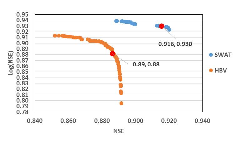
Figure 6. Non-dominated trade-offs for HBV and SWAT using PA-DDS Calibration method.

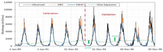
Figure 7. Hydrograph in calibration and validation periods using PA-DDS method for HBV and SWAT models.

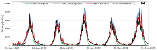
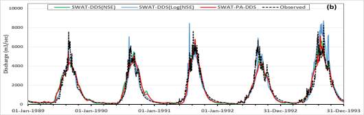
Figure 8. Hydrographs of best solution using DDS and PA-DDS for (a) HBV and (b) SWAT.

Capturing Variability or Seasonality

The analysis discussed in section 4.1 was made using the full daily hydrograph. To investigate more the differences between the two models, the ability of the model to capture the low flows and high flows is assessed separately. For this purpose, the optimal solution of PA-DDS is used because it showed better performance compared to DDS for both models as mentioned in section 4.1. The low flows and high flows were separated based on 25% of the year high values are considered high flows (Q 25%) and the remaining are low flows (Q 75%) (See figure 7). Then the low and high flows are evaluated using NSE for calibration and validation periods of the two models. The Evaluation results are summarized in Table 2, it is clear that the NSE values are lowered compared to the performance results of the complete hydrograph. SWAT is performing better than HBV for high flows and low flows in calibration, while for validation both models show unsatisfactory results. Surprisingly, NSE value for low flow modeled by HBV is better than SWAT and better than the calibration results of HBV. That could be because of the exceptional oscillations in the observed low flows in the last 3 years of validation (see figure 5) which are difficult to be matched by the smoother hydrograph produced by SWAT.

Table 2. Summary of model evaluation results for capturing variability.

	NSE
	High flows (Q25%)		Low flows (Q75%)
	SWAT	HBV	SWAT	HBV
Calibration	0.72	0.62	0.72	0.58
Validation	0.50	0.42	0.56	0.67

Model Performance Evaluation at Multiple Time-Scales

For some applications (e.g. water resources management) the interest in flows may be on higher temporal scales, that likely to be in the Nile basin where data availability is an issue. So it is important to compare and evaluate the results of the two models on different time scales. The time series of the best optimal solution of PA-DDS was used for this evaluation. This time series was aggregated on higher time scales (i.e. weekly, monthly, and annually), then compared with the aggregated observation using NSE values for the total period (1989-1998).

Figure 9 shows the simulated and observed hydrographs on different time scales and the results of NSE. The aggregation of flows on higher scale smoothed the hydrograph which improved NSE values for both HBV and SWAT. NSE value improved from 0.84 and 0.86 at the daily time scale to 0.89 and 0.92 at the monthly scale for HBV and SWAT respectively. Also on the annual scale (see Figure 9d) the two models show good results compared to observations.

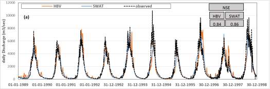
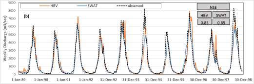
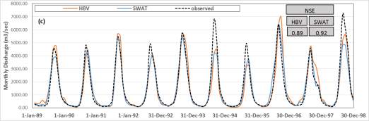
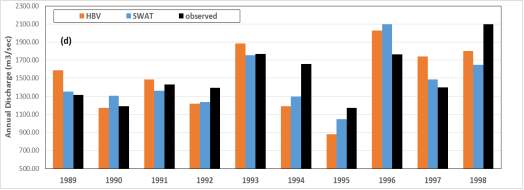
Figure 9. Simulated and observed flows at different temporal scales (a) daily, (b) weekly, (c) monthly, and (d) annually.

Conclusions

Hydrological models are important tools that are used to support proper management decisions. There is a huge number of hydrological models that were developed. These models vary in their physical representation and discretization. It is indefinite which of these models is the best to use. As a respond to this issue, this   study introduced a methodology to compare between two models that are different in terms of physical representation and discretization. SWAT which is a complex semi-distributed physical model and HBV which is a simple conceptual lumped model. The two models were evaluated based on their ability to simulate the observation at the outlet of a case study basin (UBNB). The results of the calibration of both models were very good. The value of NSE for both models exceeded 90% during calibration and 83% during validation when the two models calibrated using DDS with NSE as objective function. The calibration using DDS was repeated by using log(NSE) as objective function and the results remained very good with better representation for the low flows compared to the case of using NSE as objective function. The calibration was also carried out using two-objective functions algorithm (PA-DDS) with NSE and log(NSE) as objective functions. The results of PA-DDS for both models showed better matching hydrographs for high and low flows when evaluated visually. However, the overall performance evaluated by NSE and log(NSE) values were slightly lower than the results of DDS.

The resulted best optimal solution of PA-DDs calibration method was used to evaluate the ability of the model to capture the seasonality in observations. The results showed good NSE values for HBV and SWAT for high and low flow during calibration. But the results were unsatisfactory during validation period, which indicates that the goodness of the overall performance measures does not necessarily mean that the model captures well the low and high flow values. The resulted hydrograph of PA-DDs calibration was used also to compare the hydrograph on different time scales with observations. The results showed good performance for both models. With slightly higher NSE values for SWAT.

It can be inferred that HBV showed a comparable performance to SWAT when evaluated based on the ability to simulate the observations at the outlet of UBNB. The complexity of structure, methods, and discretization of SWAT seems to give the model a slightly better performance metric values. For practicality, HBV can be considered better option to simulate flows at single outlet, because it takes lesser time and effort in terms of model setup and computations, also needs less data. To reach more robust conclusions a population-based algorithm for calibration should be used to minimize the likelihood of getting local optimum solution for calibration. Also, the analysis should be done on the ensemble of results not only on the best solution.

REFERENCES

Arnold, J. G., Allen, P. M., & Bernhardt, G. (1993). A comprehensive surface-groundwater flow model. Journal of Hydrology, 142(1–4), 47–69. https://doi.org/10.1016/0022-1694(93)90004-S

Arnold, J. G., Srinivasan, R., Muttiah, R. S., & Williams, J. R. (1998). Large area hydrologic modeling and assesment Part I: Model development. JAWRA Journal of the American Water Resources Association, 34(1), 73–89. https://doi.org/10.1111/j.1752-1688.1998.tb05961.x

Asadzadeh, M., & Tolson, B. A. (2009). A New Multi-Objective Algorithm , Pareto Archived DDS. 11th Annual Conference Companion on Genetic and Evolutionary Computation Conference, 1963–1966. https://doi.org/10.1145/1570256.1570259

Bergstrom, S. (2014). List of publications and documents on research on and applications of the HBV model. Retrieved from https://hepex.irstea.fr/the-hbv-model-40-years-and-counting/

Betrie, G. D., Mohamed, Y. A., Van Griensven, A., & Srinivasan, R. (2011). Sediment management modelling in the Blue Nile Basin using SWAT model. Hydrology and Earth System Sciences, 15(3), 807–818. https://doi.org/10.5194/hess-15-807-2011

Beven, K., & Freer, J. (2001). Equifinality, data assimilation, and uncertainty estimation in mechanistic modelling of complex environmental systems using the GLUE methodology. Journal of Hydrology, 249(1–4), 11–29. https://doi.org/10.1016/S0022-1694(01)00421-8

Bontemps, S., Defourny, P., Bogaert, E. V., Arino, O., Kalogirou, V., & Perez, J. R. (2011). GLOBCOVER 2009-Products description and validation report, (September 2014), 7400.

Conway, D. (1997). A water balance model of the Upper Blue Nile in Ethiopia. Hydrological Sciences Journal-Journal Des Sciences Hydrologiques, 42(2), 265–286. https://doi.org/10.1080/02626669709492024

Dile, Y. T., & Srinivasan, R. (2014). Evaluation of CFSR climate data for hydrologic prediction in data-scarce watersheds: An application in the blue nile river basin. Journal of the American Water Resources Association, 50(5), 1226–1241. https://doi.org/10.1111/jawr.12182

Fuka, D. R., Walter, M. T., Macalister, C., Degaetano, A. T., Steenhuis, T. S., & Easton, Z. M. (2013). Using the Climate Forecast System Reanalysis as weather input data for watershed models. Hydrological Processes, 28(22), 5613–5623. https://doi.org/10.1002/hyp.10073

Green, W., & Ampt, G. (1911). Studies on soil physics, the flow of air and water through soils. The Journal of Agricultural Science, 4, 1–24.

Hargreaves, G. L., Hargreaves, G. H., & Riley, J. P. (1985). Agricultural Benefits for Senegal River Basin. Journal of Irrigation and Drainage Engineering, 111(2), 113–124. https://doi.org/10.1061/(ASCE)0733-9437(1985)111:2(113)

Kim, U., Kaluarachchi, J. J., & Smakhtin, V. U. (2008). Generation of monthly precipitation under climate change for the upper Blue Nile River Basin, Ethiopia. Journal of the American Water Resources Association, 44(5), 1231–1247. https://doi.org/10.1111/j.1752-1688.2008.00220.x

Lehner, B., Verdin, K., & Jarvis, A. (2006). HydroSHEDS Technical Documentation. Washington, DC.: World Wildlife Fund US. Retrieved from https://hydrosheds.cr.usgs.gov/

Lindström, G., Johansson, B., Persson, M., Gardelin, M., & Bergström, S. (1997). Development and test of the distributed HBV-96 hydrological model. Journal of Hydrology, 201(1–4), 272–288. https://doi.org/10.1016/S0022-1694(97)00041-3

Liu, Ben M. , Collick, Amy S. , Zeleke, Gete , Adgo, Enyew , Easton, Zachary M. , Steenhuis, T. S. (2008). Rainfall-discharge relationships for a monsoonal climate in the Ethiopian highlands. Hydrological Processes, 22, 1059–1067. https://doi.org/10.1002/hyp.7022

Monteith, J. L. (1965). Evaporation and environment. Symposia of the Society for Experimental Biology. https://doi.org/10.1613/jair.301

Neitsch, S. L., Arnold, J. G., Kiniry, J. R., & Williams., J. R. (2005). Soil and Water Assessment Tool Theoretical Documentation Version 2005. United States Department of Agriculture, Agricultural Research Service. Retrieved from http://swat.tamu.edu/media/1292/swat2005theory.pdf

Priestley, C. H. B., & Taylor, R. J. (1972). On the Assessment of Surface Heat Flux and Evaporation Using Large-Scale Parameters. Monthly Weather Review, 100(2), 81–92. https://doi.org/10.1175/1520-0493(1972)100<0081:OTAOSH>2.3.CO;2

Rientjes, T. H. M., Haile, A. T., Kebede, E., Mannaerts, C. M. M., Habib, E., & Steenhuis, T. S. (2011). Changes in land cover, rainfall and stream flow in Upper Gilgel Abbay catchment, Blue Nile basin – Ethiopia. Hydrology and Earth System Sciences, 15(6), 1979–1989. https://doi.org/10.5194/hess-15-1979-2011

Sutcliffe, J. V., & Parks, Y. P. (1999). The Hydrology of the Nile. IAHS Special Publication, 5(5), 192.

Tolson, B. A., & Shoemaker, C. A. (2007). Dynamically dimensioned search algorithm for computationally efficient watershed model calibration. Water Resources Research, 43(1), 1–16. https://doi.org/10.1029/2005WR004723

USDA. (1972). USDA Soil Conservation Service.National Engineering Handbook, Section 4.

van Engelen, V. W. P., & Dijkshoorn, J. a. (2013). Global and National Soils and Terrain Digital Databases (SOTER). Procedures Manual, Version 2.0, 198. Retrieved from http://www.isric.org/projects/soil-and-terrain-soter-database-programme

Woldesenbet, T., Elagib, N., Ribbe, L., & Heinrich, J. (2017). Hydrological responses to land use / cover changes in the source region of the Upper Blue Nile Basin , Ethiopia. Science of the Total Environment, 575, 724–741. https://doi.org/10.1016/j.scitotenv.2016.09.124