Gas Generator System for Jet Acoustic Facility
Info: 19502 words (78 pages) Dissertation
Published: 11th Dec 2019
A gas generator, a device for generating gas and also may be used to drive a turbine or to create gas from pressurized gas source when storing a solid or liquid is undesirable or impractical. The term often refers to a device that uses a rocket propellant to generate large quantities of gas that is typically used to drive a turbine and also to provide thrust as in a rocket engine. In aero acoustics, jet noise is the field that focuses on the noise generation caused by high-velocity jets, such noise is known as broadband noise and extends well beyond the range of human hearing and is also responsible for some of the loudest sounds ever produced by mankind. The upper stage of GSLV MkIII the next generation launch vehicle of ISRO is powered by a cryogenic engine called CE-20. The engine is first of its kind that works in gas generator cycle. CE-20 engine works on “Gas Generator Cycle” The generator system requires a Spark Plug for delivering electric current from an ignition system to the combustion chamber of a spark-ignition engine to ignite the compressed fuel/air mixture by an electric spark, while containing combustion pressure within the engine and an electro-pneumatic action valve that is a control system for pipe organs, whereby air pressure, controlled by an electric current and operated by the keys of an organ console, opens and closes valves within wind chests, allowing the pipes to speak. A thermocouple, dependent on temperature, and finally a pressure transducer, often called a pressure transmitter, a transducer that converts pressure into an electrical signal. The project aims to synchronize all the four components so that they work in sync with a minimum latency to meet the needs of the jet acoustic facility. Thus, maintaining a constant Mach number and thrust of the GSLV-M3. The cold flow and hot flow tests results will be useful in comparing and arriving at a reasonable estimate for the actual scale
CONTENTS
Abstract i
Contents ii
List of Figures v
List of Tables vi
SDSC SHAR vii
- Introduction 1-11
- Aim of the project 1
- Realization Of The Project
- Literature Survey 2-3
- GSLV Mark III 2
- Cryogenic Engine 4
- Gas Generator 4-15
- 1:100 Hot Flow Test Facility 4
- Elements of Gas Generator 4
- Air Supply Unit 5
- Combustion Chamber 5
- Kerosene Injector Assembly 6
- Acetylene Injector Assembly 7
- Cooling Water System 8
- Pneumatic System 9
- Air Supply System 9
- Kerosene Supply system 10
- Gas Generator Ignition 11
- Acetylene Ignition 11
- Bypass ignition 12
- Main Ignition 12 14
- Pipes And Instrumentation Diagram 16-18
- Operational Sequence 18
- Working
- PIC Microcontroller 19-22
- PIC18F87K22 19
- Special Microcontroller Features
- Peripheral Highlights
- PIC Microcontroller Kit 20
- System Specifications
- Mikro Bus
- ADC Click
- UART Via RS-232
- LCD 2×16
- GLCD 128×64
- LM-35
- Output Voltages
- Transducers 32-35
- Thermocouple Type K 32
- Electro Pneumatic Valve 33
- Spark Plug 34
- Pressure Transducer 35
- Software Requirements
- Python
- Python IDLE
- Raspberry Pi
- Graphical User Interface
- Proteus Design Suite
- Sequence For Execution
- MP Lab IDE
- Sequence Of Steps
- Mikro Program Suite
- Mikro C
- Simulation & Synthesis Results 37-59
- Proteus Simulation 37
- Python Simulation 52
- PIC assembly Code 59
- Conclusion 60
- References 61
- Temperature Valves & Mixture Ratio 64
LIST OF FIGURES
Figure No. Description Page No.
Fig 2.1 GSLV M3 2
Fig 2.2 Cryogenic Engine 4
Fig 3.1 Gas Generator 6
Fig 3.2 Combustion Chamber 6
Fig 3.3 Injector Assembly 7
Fig 3.4 Injector Parts 7
Fig 3.5 Flame Tube 8
Fig 3.6 Air Chamber 10
Fig 3.7 Assembled View of Kerosene Injector 15
Fig 3.8 Injector Assembly Mount On Main Header 15
Fig 4.1 P&I Diagram Of Gas Generator 18
Fig 5.1 PIC 18F87K22 21
Fig 5.2 PIC Block Diagram 22
Fig 6.1 PIC Pro Kit 23
Fig 6.2 Dual Power Supply Unit 24
Fig 6.3 Dual Power Supply Schematics 24
Fig 6.4 Mikro Bus Female 25
Fig 6.5 Mikro Bus Male 25
Fig 6.6 Mikro Bus Pin Description 26
Fig 6.7 ADC Click 27
Fig 6.8 ADC Click schematic 27
Fig 6.9 RS 232 28
Fig 6.10 LCD 28
Fig 6.11 LCD connector 29
Fig 6.12 LCD Pins 29
Fig 6.13 GLCD 30
Fig 6.14 GLCD Pins 30
Fig 6.15 LM 35 31
Fig 6.16 Output Voltage Terminal 31
Fig 7.1 Thermocouple junctions 32
Fig 7.2 Thermocouple Block Diagram 32
Fig 7.3 Thermocouple Reference 33
Fig 7.4 Pneumatic Valves 34
Fig 7.5 Spark Plug 35
Fig 7.6 Pressure Transducer 35
Fig 7.7 Pressure Transducer Model 36
Fig 8.1 UART Sender 37
Fig 8.2 LCD 38
Fig 8.3 ADC 39
Fig 8.4 GLCD 42
Fig 8.5 ADC On UART 44
Fig 8.6 LM 35 48
Fig 8.7 Horizontal Valve 50
Fig 8.8 Flame 1 50
Fig 8.9 Flame 2 50
Fig 8.10 Flame 3 51
Fig 8.11 Valve 51
Fig 8.12 Valve 1 51
Fig 8.13 Valve 2 51
Fig 8.14 Sparkn2 51
Fig 8.15 Sparkn 51
Fig 8.16 Spark 51
Fig 8.17 Vertivalve 51
Fig 8.18 Spark 51
Fig 8.19 Picture1 52
Fig 8.20 Python Logo 73
LIST OF TABLES
Table No. Description Page No.
Table 1 Features Of PIC18 Family 20
Table 2 Thermocouple Voltages(mv) 33
SDSC SHAR
About SDSC SHAR :
Sriharikota, a remote inaccessible island, was acquired in the year 1969 to establish a national range for launching of multistage rockets and satellite launch vehicles. Features like nearness to the Equator, largely uninhabited island, and good launch azimuth corridor for various missions, situated on the east coast of India, identifies SHAR as an ideal spaceport. Sriharikota is located 18 km east of Sullurupeta, a small town on Chennai – Kolkata National Highway between Nellore and Chennai. Sriharikota covers an area of about 43,360 acres (175 sq.km) with a coastline of 50 km.
SHAR, popularly known as “Spaceport of India”, is located at Sriharikota a spindle shaped island. This space centre was renamed as Satish Dhawan Space Centre SHAR on September 5, 2002 in memory of Prof. Satish Dhawan, former Chairman of the Indian Space Research Organisation (ISRO)
SDSC SHAR embarked its journey into space by launching RH-125 from Sriharikota on October 9, 1971. Launch facilities were set up in early eighties, for the first generation ISRO satellite launch vehicles, namely SLV-3 and ASLV. SDSC SHAR houses the necessary infrastructure for launching sounding rockets, satellite launch vehicle missions (PSLV/ GSLV/ LVM3) to Low Earth Orbit (LEO), Sun Synchronous Orbit (SSO), Geosynchronous Transfer Orbit (GTO), controlled reentry missions & deep space missions.

About SMP & ETF :
Solid Motor Performance and Environmental Test Facilities (SMP & ETF) is mainly responsible for conducting static testing of solid rocket motors, both at sea-level and simulated high altitude conditions. It also caters to the environmental testing requirements of solid rocket motors and their subsystems which include Vibration, Shock, Constant Acceleration, and Thermal/Humidity. The following are the test facilities:-
Sea-level Static Test Facilities
High Altitude Test Facility
Vibration Test Facility
Thermal Soak & Humidity Test Facility
Constant Acceleration Test Facility
Aero Acoustic Test Facility (AATF)
Proof Pressure Test Facility
For Sea level static Testing, Single component and six component test stands are designed and developed in house to measure the axial thrust and side force components. The rocket motors are extensively instrumented to measure various parameters such as chamber pressure, axial thrust, and temperature on motor case and nozzle and strain, etc.
High Altitude Test Facility is meant for simulating high altitude vacuum conditions for testing upper stage rocket motors. In this high altitude test facility Vacuum ignition of motor, Motor subsystem performance in vacuum, Nozzle qualification for full flow conditions and Motor tail-off thrust characteristics are validated.
In vibration test facility, an electro-dynamic shaker is used for testing of rocket motor and their subsystems by simulating required longitudinal and later vibration.
Simulating low temperature, high temperature, temperature cycling and different humidity conditions on the rocket motors and their subsystems is carried out in Thermal Soak & Humidity Test Facility.
Simulating acceleration loads on the rocket motor is conducted at Constant Acceleration Test Facility.
Aero Acoustic Test Facility (AATF) is used for simulating the acoustic levels during liftoff of the launch vehicle. Water injection system has been employed to suppress the acoustic levels, the water injection parameters like injection pressure, location of injection, angle of injection, mass flow rate of water has been extensively studied for suppressing the acoustic loads.
As part of qualification programme Proof Pressure test or burst tests are conducted on newly realized hardware or to gain confidence of an old hardware or even to evaluate the failure mode of the hardware.
CHAPTER 1
INTRODUCTION
To establish the acoustic characteristics of GSLV-M3 during its lift-off from SLP, cold flow model tests are being conducted at present using 1:100 scale with Nitrogen as driving fluid. From the literature, it is learnt that heated jets and its acoustic characteristics need to be studied for understanding the Strouhal number criterion and also the exit location of water injection in order to achieve better attenuation levels. The length of the potential cores will be different for the cold and hot supersonic over expanded jets. To achieve optimum attenuation level water is to be injected at the end of the potential core. Further, difference in acoustic level of two jets with same velocities for different temperatures occurs at low frequencies. However from the literature it is learnt that the attenuation levels will be more or less the same for cold and hot jets.
It is proposed to study the acoustic characteristics of heated supersonic jets and the effect of water injection on the suppression characteristics at various nozzle exit velocities keeping the Mach number constant by varying stagnation temperatures. It is planned to conduct this test for the scale down model of 1:100, where mass flow requirement is comparatively less. A Gas Generator system operating with kerosene-air mixture has been realized to generate heated air at 30bar and a temperature range of 600K to 1200K. This report details the Gas generator system and its remote operation.
1.1 Aim of Project
The objective of the project is to operate the Gas Generator System Remotely through an embedded system. As the system is being designed for test module it requires to be changed a multiple times to conduct tests for different parameters and different environments, hence a microcontroller is being used. These tests would provide vital inputs for the forthcoming hot flow model tests using scaled solid rocket motors simulating S200 motors of gsLVM3. Finally, it should be ensured that the working is done with minimum or no delay if feasible. The components in play should be well synced with a proper fluidic flow of code and data acquisition.The GUI should be displayed well so as to facilitate efficient monitoring.
1.2 Realization Of The Project
The project is done using a PIC microcontroller and the GUI is displayed on the Python. The transducers used are synced to the controller using an A/D driver. The output is given to the Relays to achieve the required voltage. The simulation is done using the Proteus 8.6 software driven by the MikroC code. The PIC and the Raspberry Pi can be interfaced to run the process and the GUI simultaneously. The progress is displayed on the LCD and the GLCD of the microcontroller kit. Microcontroller is a better choice when compared to PLC as the project is the downscaled testing version of the gas generator and is easily manipulated. The graphs saved will help in further estimations and calculations of the CE-20 engine.
CHAPTER 2
LITERATURE SURVEY
2.1 Geosynchronous Satellite Launch Vehicle Mark III:
The Geosynchronous Satellite Launch Vehicle Mark III , also referred to as the Launch Vehicle Mark 3, LVM3 or GSLV-III is a launch vehicle developed by the Indian Space Research Organisation (ISRO).
It is intended to launch satellites into geostationary orbit and as a launcher for an Indian crew vehicle. The GSLV-III features an Indian cryogenic third stage and a higher payload capacity than the current GSLV
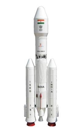
Figure 2.1:GSLV
Vehicle description:-
First Stage:
The S200 solid motors are used as the first stage of the launch vehicle. Each booster has a diameter of 3.2 metres, a length of 25 metres, and carries 207 tonnes of propellant. These boosters burn for 130 seconds and produce a peak thrust of about 5,150 kilonewtons (525 ft) each.
A separate facility has been established at Sriharikota to make the S200 boosters. Another major feature is that the S200’s large nozzle has been equipped with a ‘flex seal.’ The nozzle can therefore be gimballed when the rocket’s orientation needs correction.
In flight, as the thrust from the S200 boosters begins to tail off, the decline in acceleration is sensed by the rocket’s onboard sensors and the twin Vikas engines on the ‘L110’ liquid propellant core stage are then ignited. Before the S200s separate and fall away from the rocket, the solid boosters as well as the Vikas engines operate together for a short period of time.
Second Stage
The second stage, designated L110, is a 4-meter-diameter liquid-fueled stage carrying 110 tonnes of UDMH and N2O4. It is the first Indian liquid-engine cluster design, and uses two improved Vikas engines, each producing about 700 kilonewtons (70 tf).The improved Vikas engine uses regenerative cooling, providing improved weight and specific impulse, compared to earlier rocketsThe L110 core stage ignites 113 seconds after liftoff and burns for about 200 seconds.
Third Stage
The cryogenic upper stage is designated the C25 and will be powered by the Indian-developed CE-20 engine burning LOX and LH2, producing 186 kilonewtons (19.0 tf) of thrust. The C-25 will be 4 metres (13 ft) in diameter and 13.5 metres (44 ft) long, and contain 27 tonnes of propellant.
This engine was initially slated for completion and testing by 2015, it would have been the C25 stage and be put through a series of tests. ISRO crossed a major milestone in the development of CE-20 engine for the GSLV MKIII vehicle by the successful hot test for 640 seconds duration on 19 February 2017 at ISRO Propulsion Complex, Mahendragiri. The test demonstrated the repeatability of the engine performance with all its sub systems like thrust chamber, gas generator, turbo pumps and control components for the full duration. All the engine parameters were closely matching with the pre-test prediction.
The first C25 stage will be used on the GSLV-III D-1 missionin December 2016. This mission will put in orbit the GSAT-19E communication satellite. Work on the C25 stage and CE-20 engine for GSLV Mk-III upper stage was initiated in 2003, the project has been subject to many delays due to problems with ISRO’s smaller cryogenic engine, the CE-7.5 for GSLV MK-II upper stage.
Comparable rockets
- Angara A3
- Delta IV
- Falcon 9
- H-IIA
- Long March 3B
- Titan IIIC
2.2Cryogenic Engine for GSLV MkIII
The upper stage of GSLV MkIII the next generation launch vehicle of ISRO is powered by a cryogenic engine called CE-20. This engine produces a nominal thrust of 200 kN, but has an operating thrust range between 180 kN to 220 kN and can be set to any fixed values between them.The engine is first of its kind that works in gas generator cycle and indigenously developed. The combustion chamber burns liquid hydrogen and liquid oxygen at 6 MPa with 5.05 engine mixture ratio. The engine has a thrust-to-weight ratio of 34.7 and a specific impulse of 443 seconds in vacuum. ISRO successfully tested the sea level version of the engine for a cumulative duration of about 1900 s spread over ten hot tests which includes flight duration hot test of 635s on April 28, 2015 and endurance hot test for duration of 800 seconds. CE-20 engine works on “Gas Generator Cycle” which has flexibility for independent development of each sub-system before the integrated engine test, thus minimising uncertainty in the final developmental phase with reduced development time. The high thrust cryogenic engine is one of the most powerful upper stage cryogenic engines in the world. Starting with injector element development for configuration of injector head, the design, realization and testing of the major subsystems viz the gas generator, turbo pumps, start-up system and thrust chamber, have been successfully completed in a phased manner before conducting a series of developmental tests in the integrated engine mode. Apart from the major sub-systems, many critical components like the igniter, control components etc were independently developed and qualified
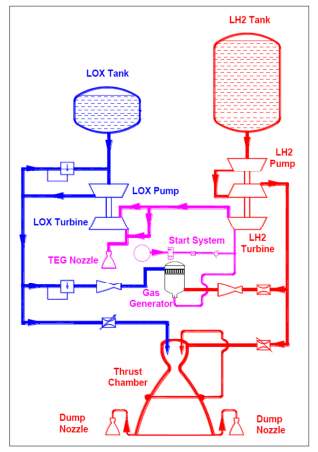
Figure 2.2: Cryogenic Engine Schematic Diagram
CHAPTER 3
GAS GENERATOR
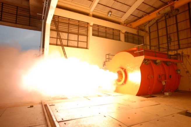
Gas Generator is nothing but a can type combustor operating with kerosene-air mixture, which caters heated air at desired pressure, temperature and mass flow rate for hot flow model test. During the ignition phase, pilot flame is established by means of acetylene gas, which is ignited through a high voltage spark source.
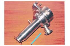
Figure 3.1 Gas Generator
3.1 Elements Of Gas Generator
The Gas Generator consists of the sub-systems like Air supply unit, Combustion Chamber, Kerosene Injector assembly, Acetylene Injector assembly, Flame holder tube, Igniter assembly and Cooling water system. Air supply unit is a cylindrical shell, which receives the air from the main air line and supplies to the combustion chamber. Combustion chamber is a cylindrical shell, where the actual combustion takes place.
3.1.1 1:100 Hot Flow Test Facility for studying GSLV-M3 Lift-off
Kerosene Injector is the one, which supplies the kerosene to the combustion chamber. There are 3 injectors mounted on a header at the center of the combustion chamber. Acetylene injector is the one, which supplies acetylene gas for providing pilot flame inside the chamber. Flame holder tube is a divergent conical passage, which has perforations all around for uniform distribution of air in turn resulting in better mixing in the combustion chamber. It acts as a flame holding unit through aerodynamic flame stabilization. Igniter assembly is mounted on the combustion chamber and its tip is mounted aside the acetylene injector with a small gap of 1mm maintained between them.
Cooling water system is a Jacket type cooling system, i.e. the combustion chamber is surrounded by another cylindrical shell to cool the combustion chamber. Water is circulated once through for effective cooling in counter flow direction.
3.2.2 Air Supply Unit
Air Chamber is a cylindrical shell , which receives the air from the main air line and supplies to the combustion chamber. The regulated air supply from the proportional control valve is fed to the air chamber.
3.2.3 Combustion Chamber
Combustion chamber is a cylindrical shell, where through mixing of kerosene and air takes place. Combustion chamber flange has a step on its face to hold the flame tube
3.2.4 Kerosene Injector assembly
The kerosene injectors are mounted on a toroid, which in turn is connected to the kerosene supply line. The injectors are meant for supplying the kerosene into the combustion chamber in a finely atomized state. The injectors used are simplex type injectors or Pressure- swirl injectors. In this injector, the kerosene is caused to swirl by tangential slots.
3.2.5 Acetylene Injector Assembly
The acetylene injector assembly is mounted in the combustion chamber exactly at the center of the kerosene injector assembly. The acetylene is supplied by this injector at a pressure of 0.2 bar for the initial ignition phase for establishing the pilot flame.
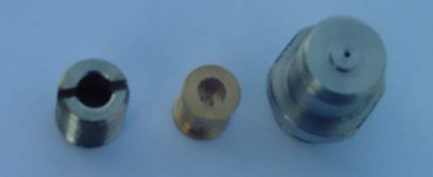
Fig. 3.4: Injector Parts
3.2.6 Flame Tube
The flame tube is a divergent conical passage, which has perforations all around for uniform distribution of air in the combustion chamber. The flame tube is designed in such a way that it sustains at higher combustion temperatures.
The flame tube is divided into three zones along the flow direction, they are called as
- Primary zone
- Intermediate zone
 Dilution zone
3.2.7 Cooling Water System
Cooling water system is a Jacket type cooling system, i.e. the combustion chamber is surrounded by another cylindrical shell in which water flows continuously to cool the combustion chamber.
3.3 PNEUMATIC SYSTEM
The pneumatic system comprises of the
- Air supply system
- Kerosene supply system
- Acetylene supply system
3.3.1Air supply system
Air is supplied to the Gas Generator at 300bar pressure. Air from the 300bar storage module is regulated to a operating pressure of 30bar by means of a pressure regulator.
3.4 Kerosene supply system
This system pressurizes kerosene by means of Nitrogen to 45 bar and supplies the kerosene to the combustion chamber though a proportional control valve. Kerosene is stored in a storage tank.
3.4.2 Requirement of N2
Nitrogen gas is used to pressurize kerosene to a pressure of 45 bar. Nitrogen is stored at 300bar pressure and it is regulated to operating pressure of 45bar by means of a pressure regulator.
3.5 GAS GENERATOR IGNITION
It is planned to operate the Gas Generator in remote mode using electro -pneumatic valves and proportional control valves as shown in the P&I diagram. The gas generator operation is carried out in three phases as below;
Phase –I : Acetylene Ignition
- Phase –II : By-Pass Ignition (Air at 5bar)
- Phase –III : Main Ignition (Air at 30bar)
3.5.1 Phase I-Acetylene Ignition
For initial ignition purpose acetylene is used to fire the kerosene air mixture. For this acetylene is sent to the combustion chamber through a electro pneumatic valve at 0.2bar pressure. Acetylene is ignited by an igniter, which supplies sparks continuously from a high voltage source. The Air/Fuel Ratio for acetylene is reported to be12.14.
3.5.2 Phase II-Bypass Ignition
In the Acetylene ignition phase, once the acetylene flame is stabilized then the Kerosene proportional control valve is operated to supply kerosene into the combustion chamber. Subsequently the By Pass air-line valve is opened which supplies air The kerosene is supplied to the combustion chamber ,Once kerosene air mixture catches fire, the acetylene flame is put-off.
3.5.3 Phase –III Main Ignition
In the bypass mode, once the flame stabilizes the kerosene proportional control valve is operated to a position corresponding to flow of kerosene flow and then the main air line valve is operated to allow air at 30bar pressure. Subsequently the bypass air-line valve is closed.
CHAPTER 4
PIPES AND INTRUMENTATION DIAGRAM
A piping and instrumentation diagram/drawing (P&ID) is a detailed diagram in the process industry which shows the piping and vessels in the process flow, together with the instrumentation and control devices.
Superordinate to the piping and instrumentation flowsheet is the process flow diagram (PFD) which indicates the more general flow of plant processes and equipment and relationship between major equipment of a plant facility.
A piping and instrumentation diagram/drawing (P&ID) is defined by the Institute of Instrumentation and Control as follows:
A diagram which shows the interconnection of process equipment and the instrumentation used to control the process. In the process industry, a standard set of symbols is used to prepare drawings of processes. The instrument symbols used in these drawings are generally based on International Society of Automation (ISA) Standard S5.1
The primary schematic drawing used for laying out a process control installation.
They usually contain the following information:
- Process piping, sizes and identification, including:
- Pipe classes or piping line numbers
- Flow directions
- Interconnections references
- Permanent start-up, flush and bypass lines
- Mechanical equipment/ Process control instrumentation and designation (names, numbers, unique tag identifiers), including:
- Valves and their identifications (e.g. isolation, shutoff, relief and safety valves)
- Control inputs and outputs (sensors and final elements, interlocks)
- Miscellanea – vents, drains, flanges, special fittings, sampling lines, reducers and increasers
- Interfaces for class changes
- Computer control system
- Identification of components and subsystems delivered by others
P&IDs are originally drawn up at the design stage from a combination of process flow sheet data, the mechanical process equipment design, and the instrumentation engineering design. During the design stage, the diagram also provides the basis for the development of system control schemes, allowing for further safety and operational investigations, such as a Hazard and operability study (HAZOP). To do this, it is critical to demonstrate the physical sequence of equipment and systems, as well as how these systems connect.
P&IDs also play a significant role in the maintenance and modification of the process after initial build. Modifications are red-penned onto the diagrams and are vital records of the current plant design.
They are also vital in enabling development of;
- Control and shutdown schemes
- Safety and regulatory requirements
- Start-up sequences
- Operational understanding.
P&IDs form the basis for the live mimic diagrams displayed on graphical user interfaces of large industrial control systems such as SCADA and distributed control systems.
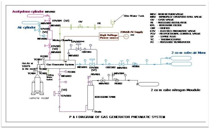
Figure 4.1:P & I Diagram of Gas Generator Pnumatic System
CHAPTER 5
OPERATIONAL SEQUENCE
The code first checks the cylinder pressures in order to check for leakages and any other hazards that might occur. The stable pressures are noted and cross checked with the optimum safe levels. The two valves are then open to let the gases into the mixing chamber where the minimum Air Fuel ratio of 12.14 is maintained Acetylene is the fuel and air is supplied to provide for combustion. After a Pressure of 60 bar is reached with the proper air fuel ration the mixture is kept at a standstill and the valves are closed. Simultaneously the Nitrogen gas valve is opened to pressurize the kerosene up to 45 bar so as to create the required thrust for the kerosene fuel. Now, the gases in the mixing chamber are let into the combustion chamber to create a pilot flame. A high voltage spark plug of 230V ac supply is used for ignition. The pilot flame is stabilized up to 1200K after which the kerosene is pumped into the chamber to create a steady flow in the gas generator. Finally the pressure readings and temperature readings are noted so as to judge the working and characteristics of the hot flow model.First the combustion temperature and the presuure flow of kerosene is kept in constant observation to ensure unhindered functioning as the kerosene gas keeps the flame alive .Next the combustion temperature and hot flow gas flame pressure is noted,thus ensuring that there is constant thrust at the output which is the main aim of this model. These observations provide the results and future inputs needed to develop the life size model made.
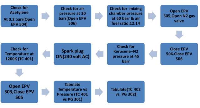
Figure 5.1 Sequence
5.1WORKING:
The Embedded C code is run on the MikroC platform and the hex file is then dumped onto the microcontroller kit. The kit is stacked with a four channel ADC driver where the inputs of the transducers are given. As needed 2 inputs and 2 for output. Then the code is run, the input voltages from the transducers are then tallied with tables according to their make and the respective values are displayed on the LCD screen. Simultaneously, the GUI is displayed in the GLCD that is mounted. The relay continues and the sequence is repeated. The output is sent to the relay switches where the voltage is amplified to meet the requirement. The valves and the spark plug require a digital output .After one cycle, the results are tabulated for future reference and the graphs are marked so as to attain a constant sloped curve.
CHAPTER 6
PIC MICROCONTROLLER
Microcontroller is a chip that combines the microprocessor with one or more other components. These components contains memory, ADC (Analog-to-Digital Converter),DAC (Digital-to-Analog Converter), parallel I/O interface, serial I/O interface, timers and counters. The microprocessor responses to arithmetically operate the binary data which likes a CPU in a computer. However, its speed, general purpose registers, memory addressing and instruction set are very low compare with a CPU. Therefore, it can be illustrated as a low level CPU. The memory is used for storing the data, programming instruction and results. It also provides these information to other units. So that the microcontroller can be processed by a pre-written instruction without computer or any other devices. The ADC and DAC can do convert signal between analog signal and digital. The analog signal usually is a voltage number in a range. Such as a temperature sensor, it can converts the temperature value to a specific voltage value. Then, this voltage value can be converted to digital value as binary via ADC. In addition, the parallel I/O interface and serial I/O interface supply one or more ports for connecting sensors on the microcontroller.The timers and counters of microcontroller provide a specific frequency. This frequency determines how process speed in this programmer.
5.1 PIC18F87K22 FAMILY
Low-Power Features:
• Power-Managed modes:
– Run: CPU on, peripherals on
– Idle: CPU off, peripherals on
– Sleep: CPU off, peripherals off
• Two-Speed Oscillator Start-up
• Fail-Safe Clock Monitor
• Power-Saving Peripheral Module Disable (PMD)
• Ultra Low-Power Wake-up
• Fast Wake-up, 1s Typical
• Low-Power WDT, 300 nA Typical
• Ultra Low 50 nA Input Leakage
• Run mode Currents Down to 5.5A, Typical
• Idle mode Currents Down to 1.7A Typical
• Sleep mode Currents Down to Very Low 20 nA,
Typical
• RTCC Current Downs to Very Low 700 nA,
Typical
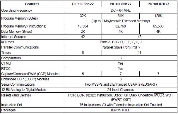
Table 1:Features of PIC18F Family
5.2 Special Microcontroller Features:
• Operating Voltage Range: 1.8V to 5.5V
• On-Chip 3.3V Regulator
• Operating Speed up to 64 MHz
• Up to 128 Kbytes On-Chip Flash Program Memory
• Data EEPROM of 1,024 Bytes
• 4K x 8 General Purpose Registers (SRAM)
• 10,000 Erase/Write Cycle Flash Program Memory, Minimum
• 1,000,000 Erase/write Cycle Data EEPROM Memory, Typical
• Flash Retention: 40 Years, Minimum
• Three Internal Oscillators: LF-INTRC (31 kHz),MF-INTOSC (500 kHz) and HF-INTOSC
• Self-Programmable under Software Control
• Priority Levels for Interrupts
• 8 x 8 Single-Cycle Hardware Multiplier
• Extended Watchdog Timer (WDT):- Programmable period from 4 ms to 4,194s (about 70 minutes)
• In-Circuit Serial Programming™ (ICSP™) via Two Pins
• In-Circuit Debug via Two Pins
• Programmable:
– BOR
– LVD
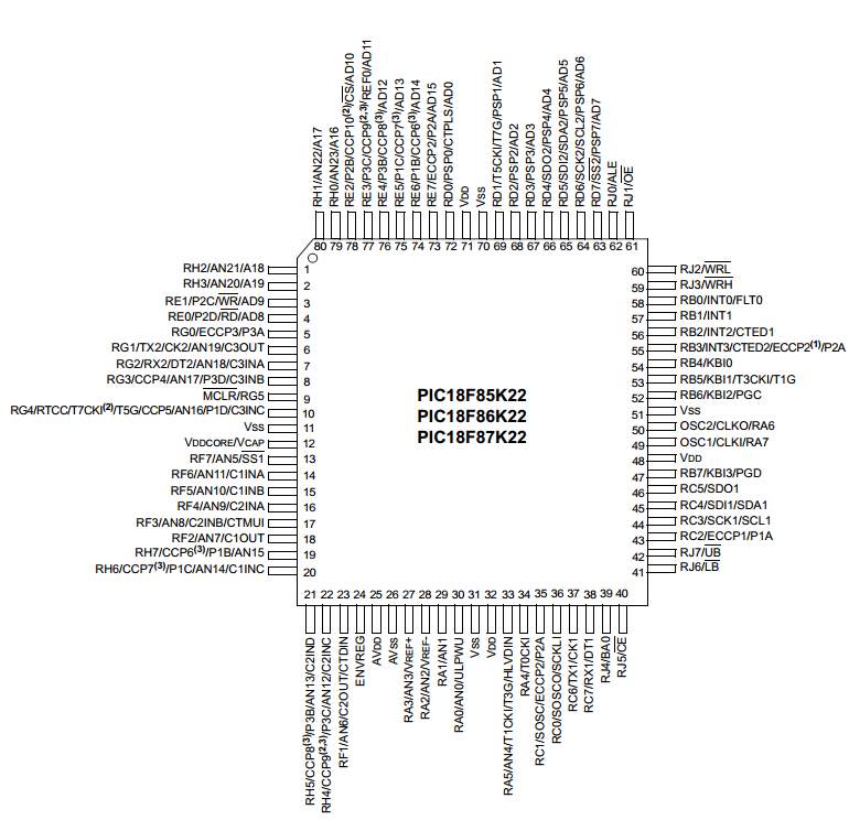
Figure 5.1 PIC18F87K22
5.3 Peripheral Highlights:
• Up to Ten CCP/ECCP modules:
– Up to seven Capture/Compare/PWM (CCP) modules
– Three Enhanced Capture/Compare/PWM (ECCP) modules
• Up to Eleven 8/16-Bit Timer/Counter modules:
– Timer0 – 8/16-bit timer/counter with 8-bit programmable prescaler
– Timer1,3 – 16-bit timer/counter
– Timer2,4,6,8 – 8-bit timer/counter
– Timer5,7 – 16-bit timer/counter for 64k and 128k parts
– Timer10,12 – 8-bit timer/counter for 64k and 128k parts
• Three Analog Comparators
• Configurable Reference Clock Output
• Hardware Real-Time Clock and Calendar (RTCC) module with Clock, Calendar and Alarm Functions
• Charge Time Measurement Unit (CTMU):
– Capacitance measurement for mTouch™ sensing solution
– Time measurement with 1 ns typical resolution
– Integrated temperature sensor
• High-Current Sink/Source 25 mA/25 mA (PORTB and PORTC)
• Up to Four External Interrupts
• Two Master Synchronous Serial Port (MSSP) modules:
– 3/4-wire SPI (supports all four SPI modes)
– I2C™ Master and Slave modes
• Two Enhanced Addressable USART modules:
– LIN/J2602 support
– Auto-Baud Detect (ABD)
• 12-Bit A/D Converter with up to 24 Channels:
– Auto-acquisition and Sleep operation
– Differential input mode of operation
• Integrated Voltage Reference
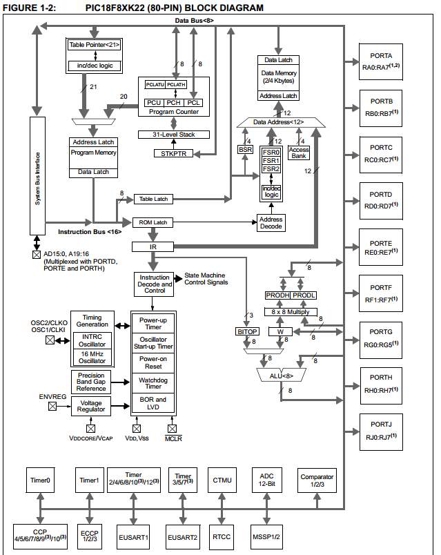
Figure 5.2 Block Diagram
PIC MICROCONTROLLER KIT
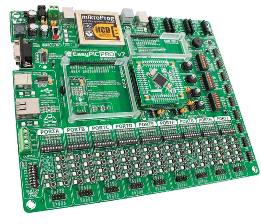
Figure 6.1 PIC Pro kit
PIC18F87K22 is the default microcontroller
it has 16 MIPS operation, 128K bytes of linear program memory, 3896 bytes of linear data memory, and support for a wide range of power supply from 1.8V to 5V. It’s loaded with great modules: 69 General purpose I/O pins, 24 Analog Input pins (AD), internal Real time clock and calendar (RTCC), support for Capacitive Touch Sensing using Charge Time Measurement Unit (CTMU), six 8-bit timers and five 16-bit timers. It also has ten CCP modules, three Comparators and two MSSP modules which can be either SPI or I 2C.

6.1 System Specification:
Power Supply : 7–23V AC or 9–32V DC or via USB cable (5V DC)
Board Dimensions : 266 x 220mm (10.47 x 8.66 inch)
Weight : 475g (1.0472 lbs)
Power Consumption : ~90mA at 5V when all peripheral modules are disconnected
Power supply
Board contains switching power supply that creates stable voltage and current levels necessary for powering each part of the board. Power supply section contains two power regulators: MC34063A, which generates VCC-5V, and MC33269DT3.3 which creates VCC-3.3V power supply, thus making the board capable of supporting both 5V and 3.3V microcontrollers. Power supply unit can be powered in two different ways: with USB power supply, and using external adapters via adapter connector (CN19) or additional screw terminals (CN18). External adapter voltage levels must be in range of 9-32V DC and 7-23V AC. Use jumper J2 to specify which power source you are using, and jumper J1 to specify whether you are using 5V or 3.3V microcontroller. Upon providing the power using either external adapter, or USB power source, you can turn the board on using SWITCH 1
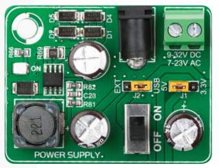
Figure 6.2:Dual power supply unit
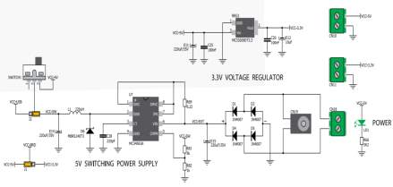
Figure 6.3:Dual power schematic
6.2 Mikrobus™
Easier connectivity and simple configuration are imperative in modern electronic devices. Success of the USB standard comes from it’s simplicity of usage and high and reliable data transfer rates. As we in MikroElektronika see it, Plug-and-Play devices with minimum settings are the future in embedded world too. This is why our engineers have come up with a simple, but brilliant pinout with lines that most of today’s accessory boards require, which almost completely eliminates the need of additional hardware settings. We called this new standard the mikroBUS™. EasyPIC PRO™ v7 is a development board which supports mikroBUS™ with three on-board sockets.
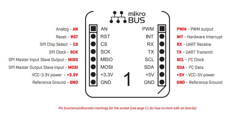
Figure 6.4:Mikrobus female
As you can see, there are no additional DIP switches, or jumper selections. Everything is already routed to the most appropriate pins of the microcontroller sockets. mikroBUS™ host connector Each mikroBUS™ host connector consists of two 1×8 female headers containing pins that are most likely to be used in the target accessory board. There are three groups of communication pins: SPI, UART and I 2C communication. There are also single pins for PWM, Interrupt, Analog input, Reset and Chip Select. Pinout contains two power groups: +5V and GND on one header and +3.3V and GND on the other 1×8 header
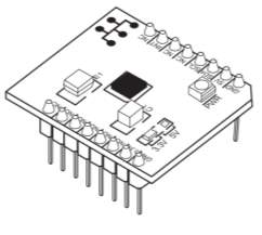
Figure 6.5:Mikrobus Male pins
The mikroBUS™ socket comprises a pair of 1×8 female headers with a proprietary pin configuration and silkscreen markings. The pinout (always laid out in the same order) consists of three groups of communications pins (SPI, UART and I2 C), six additional pins (PWM, Interrupt, Analog input, Reset and Chip select), and two power groups (+3.3V and GND on the left, and 5V and GND on the right 1×8 header). The spacing of pins is compatible with standard (100 mil pitch) breadboards
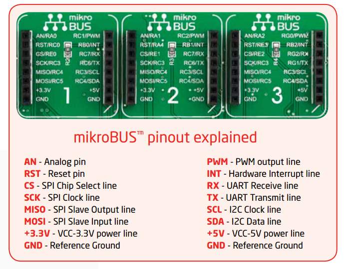
Figure 6.6:Pin description
The mikroBUS™ standard defines mainboard sockets and add-on boards used for interfacing microcontrollers or microprocessors (mainboards) with integrated circuits and modules (add-on boards). The standard specifies the physical layout of the mikroBUS™ pinout, the communication and power supply pins used, the size and shape of the add-on boards, the positioning of the mikroBUS™ socket on the mainboard, and finally, the silkscreen marking conventions for both the add-on boards and sockets. The purpose of mikroBUS™ is to enable easy hardware expandability with a large number of standardized compact add-on boards, each one carrying a single sensor, transceiver, display, encoder, motor driver, connection port, or any other electronic module or integrated circuit. Created by MikroElektronika, mikroBUS™ is an open standard — anyone can implement mikroBUS™ in their hardware design, as long as the requirements set by this document are being met.
6.3ADC click:
ADC Click is an accessory board in mikroBus™ form factor. It includes a 12-bit Analog-toDigital Converter MCP3204 that features 50k samples/second, 4 input channels and lowpower consumption (500nA typical standby, 2µA max). Board uses SPI communication interface. It is small in size and features convenient screw terminals for easier connections. Board is set to use 3.3V power supply by default. Solder PWR SEL jumper to 5V position if used with 5V systems
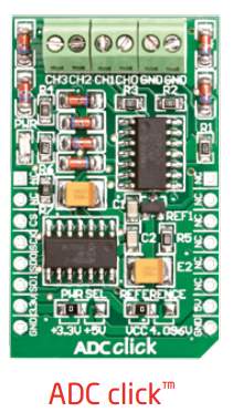
Figure 6.7:ADC click
Reading Analog Inputs
There are four analog input screw terminals for each of the supported A/D channels. We added two more terminals for GND reference. Each analog input voltage is converted to appropriate 12-bit digital value, which can be read using industry standard SPI communication interface.
SMD Jumpers
There are two zero-ohm resistors (SMD jumpers): PWR SEL is used to determine whether 5V or 3.3V power supply is used, and REFERENCE to select either VCC or 4.096V as the voltage reference.
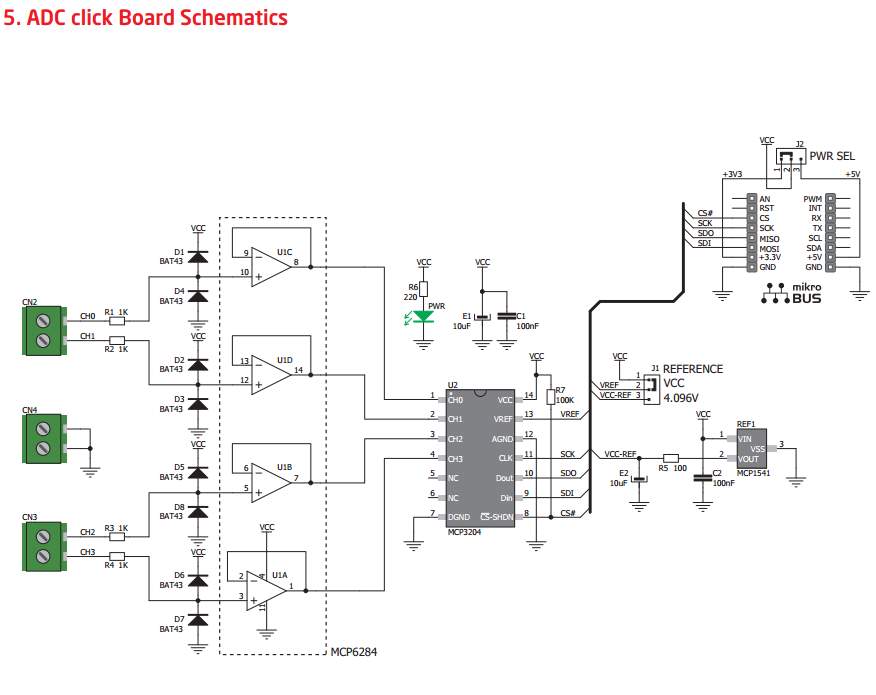
Figure 6.8:ADC click board Schematic
6.4 UART via RS-232
The UART (universal asynchronous receiver/ transmitter) is one of the most common ways of exchanging data between the MCU and peripheral components. It is a serial protocol with separate transmit and receive lines, and can be used for fullduplex communication. Both sides must be initialized with the same baudrate, otherwise the data will not be received correctly. RS-232 serial communication is performed through a 9-pin SUB-D connector and the microcontroller UART module. In order to enable this communication, it is necessary to establish a connection between RX and TX lines on SUB-D connector and the same pins on the target microcontroller using DIP switches. Since RS-232 communication voltage levels are different than microcontroller logic levels, it is necessary to use a RS- 232 Transceiver circuit, such as MAX3232
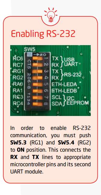
Figure 6.9:RS-232
6.5 LCD 2×16 characters
Liquid Crystal Displays or LCDs are cheap and popular way of representing information to the end user of some electronic device. Character LCDs can be used to represent standard and custom characters in the predefined number of fields. EasyPIC PRO™ v7 provides the connector and the necessary interface for supporting 2×16 character LCDs in 4-bit mode. This type of display has two rows consisted of 16 character fields. Each field is a 7×5 pixel matrix. Communication with the display module is done through CN14 display connector. Board is fitted with uniquely designed plastic display distancer, which allows the LCD module to perfectly and firmly fit into place.
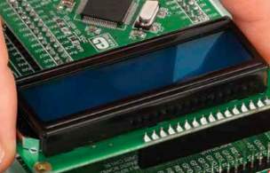
Figure 6.10:LCD
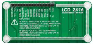
Figure 6.11:LCD Connector
Connector pinout”
GND and VCC – Display power supply lines
Vo – LCD contrast level from potentiometer P1
RS – Register Select Signal line
E – Display Enable line
R/W – Determines whether display is in Read or Write mode. It’s always connected to GND, leaving the display in Write mode all the time.
D0–D3 – Display is supported in 4-bit data mode.
D4–D7 – Upper half of the data byte
LED+ – Connection with the backlight LED anode
LED- – Connection with the backlight LED cathode
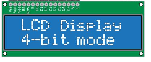
Figure 6.12:LCD pins
6.6 GLCD 128×64
Graphical Liquid Crystal Displays, or GLCDs are used to display monochromatic graphical content, such as text, images, human-machine interfaces and other content. EasyPIC PRO™ v7 provides the connector and necessary interface for supporting GLCD with resolution of 128×64 pixels, driven by the KS108 or similar display controller. Communication with the display module is done through CN16 display connector. Board is fitted with uniquely designed plastic display distancer, which allows the GLCD module to perfectly and firmly fit into place. Display connector is routed to PORTB (control lines) and PORTD (data lines) of the microcontroller sockets. Since PORTB is also used by 2×16 character LCD display, you cannot use both displays simoutaneously. You can control the display contrast using dedicated potentiometer P4. Display backlight can be enabled with SW4.2 switch, and PWM-driven backlight with SW4.3 switch.
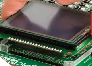
Figure 6.13:GLCD
Connector pinout
CS1 and CS2 – Controller Chip Select lines
VCC – +5V display power supply
GND – Reference ground
Vo – GLCD contrast level from potentiometer P4
RS – Data (High), Instruction (Low) selection line
R/W – Determines whether display is in Read or Write mode.
E – Display Enable line
D0–D7 – Data lines
RST – Display reset line
Vee – Reference voltage for GLCD contrast potentiometer P3
LED+ – Connection with the backlight LED anode
LED- – Connection with the backlight LED cathode
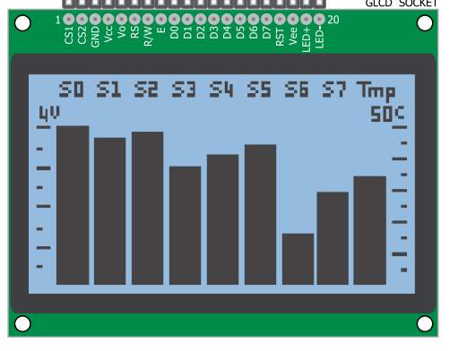
Figure 6.14:GLCD pins
6.7 LM35 – Analog Temperature Sensor
The LM35 is a low-cost precision integrated-circuit temperature sensor, whose output voltage is linearly proportional to the Celsius (Centigrade) temperature. The LM35 thus has an advantage over linear temperature sensors calibrated in ° Kelvin, as the user is not required to subtract a large constant voltage from its output to obtain convenient Centigrade scaling. The LM35 does not require any external calibration or trimming to provide typical accuracies of ±¼°C at room temperature and ±¾°C over a full -55 to +150°C temperature range. It has a linear + 10.0 mV/°C scale factor and less than 60 μA current drain. As it draws only 60 μA from its supply, it has very low self-heating, less than 0.1°C in still air. EasyPIC PRO™ v7 provides a separate socket (TS2) for the LM35 sensor in TO-92 plastic packaging. Readings are done with microcontroller using single analog input line, which is selected with a J4 jumper.
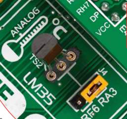
Figure 6.15:LM35
6.8 Output voltages
EasyPIC PRO™ v7 contains two additional pairs of screw terminals which can be used to get power supply output for your external devices. There are two available output voltages: 5V and 3.3V. Depending on which power source you use (adapter, laboratory power supply, or USB), maximum output currents can vary. Power consumption of the onboard modules can also affect maximum output power which can be drawn out of the screw terminals. Big power consumers, such as Ethernet, or even GLCD with backlight can alone drastically reduce the maximum output power. On-board switching power supply can give maximum of 600mA of current if used with adapter or laboratory power supply. When used with USB power supply it can give no more than 500mA. Purpose of the output voltage terminals is not to be the main power source of big consumers, but more a power source for remote small consumers.
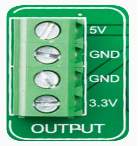
Figure 6.16: Output terminals
CHAPTER 7
TRANSDUCERS
7.1 Thermocouple Type K
Thomas Seebeck discovered if metals of two different materials were joined at both ends and one end was at a different temperature than the other, a current was created. This phenomenon is known as the Seebeck effect and is the basis for all thermocouples
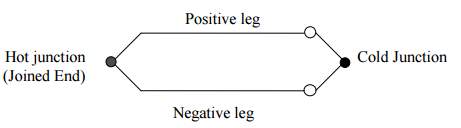
Figure 7.1:Thermcouple junctions
A thermocouple is a type of temperature sensor, which is made by joining two dissimilar metals at one end. The joined end is referred to as the HOT JUNCTION. The other end of these dissimilar metals is referred to as the COLD END or COLD JUNCTION. The cold junction is actually formed at the last point of thermocouple material
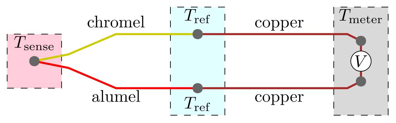
Figure 7.2: Thermocouple block dirgram
Type K:
Type K is recommended for use in oxidizing and completely inert environments. Because it’s oxidation resistance is better than Types E, J, and T they find widest use at temperatures above 1000F. Type K, like Type E should not be used in sulfurous atmospheres, in a vacuum or in low oxygen environments where selective oxidation will occur. The temperature range for Type K is -330 to 2300F and it’s wire color code is yellow and red.

Figure 7.3:Thermocouple reference
MAXIMUM TEMPERATURE RANGE:
Thermocouple Grade – 328 to 2282°F – 200 to 1250°C
Extension Grade 32 to 392°F 0 to 200°C
LIMITS OF ERROR (whichever is greater)
Standard: 2.2°C or 0.75% Above 0°C 2.2°C or 2.0% Below 0°C Special: 1.1°C or 0.4%
BARE WIRE ENVIRONMENT: Clean Oxidizing and Inert;
Limited Use in Vacuum or Reducing;
Wide Temperature Range; Most Popular Calibration
REFERENCE JUNCTION AT 0°C
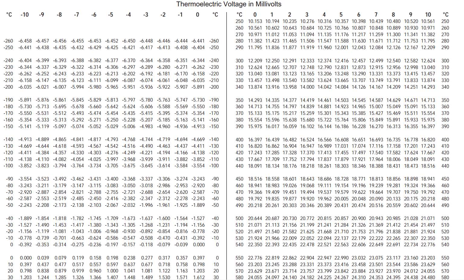
Table 2: Thermocouple Voltages
7.2 ELECTRO PNEUMATIC VALVE:
Electro-pneumatic control consists of electrical control systems operating pneumatic power systems. In this solenoid valves are used as interface between the electrical and pneumatic systems. Devices like limit switches and proximity sensors are used as feedback elements.
Seven basic electrical devices commonly used in the control of fluid power systems are
1. Manually actuated push button switches
2. Limit switches
3. Pressure switches
4. Solenoids
5. Relays
6. Timers
7. Temperature switches
Other devices used in electro pneumatics are
1. Proximity sensors
2. Electric counters
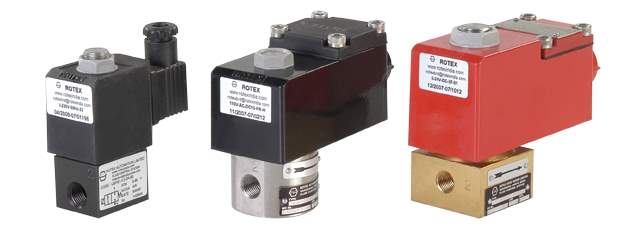
Figure 7.4:Pnumatic valves
Features :
Bubble tight shut off
Mounts in any position
Vibration resistance up to 9g
Suitable for high speed cycling
Speed up to 200 cycles/ min
Life > 5 million cycles
Media
Air, Inert Gases, Water, Free Flowing Liquids, Oil, Diesel, Kerosene, LPG, CNG
Orifice Size
25 Nominal Bore
Pressure Range(Bar)
5-400
7.3 SPARK PLUG:
A spark plug is a device for delivering electric current from an ignition system to the combustion chamber of a spark-ignition engine to ignite the compressed fuel/air mixture by an electric spark, while containing combustion pressure within the engine. A spark plug has a metal threaded shell, electrically isolated from a central electrode by a porcelain insulator. The central electrode, which may contain a resistor, is connected by a heavily insulated wire to the output terminal of an ignition coil or magneto. The spark plug’s metal shell is screwed into the engine’s cylinder head and thus electrically grounded. The central electrode protrudes through the porcelain insulator into the combustion chamber, forming one or more spark gaps between the inner end of the central electrode and usually one or more protuberances or structures attached to the inner end of the threaded shell and designated the side, earth, or ground electrode.
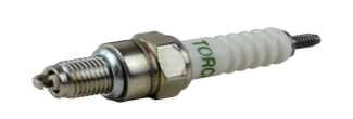
Figure 7.5:Spark Plug
Operating Voltage:24 V
Current: 0.5 A
Resistance: 80 OHM
7.4 PRESSURE TRANSDUCER:
Model Number : DRUCK UNIK 5000
The new UNIK 5000 is a high performance configurable solution to pressure measurement. The use of microma chined silicon technology and analogue circuitry enables best in class performance for stability, low power and frequency response. The new platform enables you to easily build up your own sensor to match your own precise needs. This high performance, configurable solution to pressure measurement employs modular design and lean manufacturing techniques to offer:
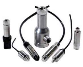
Figure 7.6:Pressure Transducer
Features
• Ranges from 70 mbar (1 psi) to 700 bar (10000 psi)
• Accuracy to ±0.04% Full Scale (FS) Best Straight Line (BSL)
• Stainless Steel construction
• Frequency response to 3.5 kHz
• High over pressure capability
• Hazardous Area certifications
• mV, mA, voltage and configurable voltage outputs
• Multiple electrical & pressure connector options
• Operating temperature ranges from –55 to 125°C (-67 to 257°F)
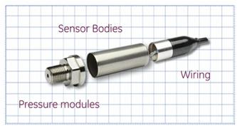
Figure 7.7:Pressure Transducer Model
Measurement:
Operating Pressure Ranges
Gauge ranges Any zero based range 70 mbar to 70 bar (1 to 1000 psi)
Sealed Gauge Ranges Any zero based range 10 to 700 bar (145 to 10000 psi)
Absolute Ranges Any zero based range 100 mbar to 700 bar (1.5 to 10000 psi)
Differential Ranges
Wet/Dry Uni-directional or bi-directional 70 mbar to 35 bar (1 to 500 psi)
Wet/Wet Uni-directional or bi-directional 350 mbar to 35 bar (5 to 500 psi)
Line pressure: 70 bar max (1000 psi)
Barometric Ranges Barometric ranges 350 mbar (5.1 psi)
CHAPTER 8
SOFTWARE REQUIREMENTS
8.1 PYTHON:
Python is an interpreted, object-oriented, high-level programming language with dynamic semantics. Its high-level built in data structures, combined with dynamic typing and dynamic binding, make it very attractive for Rapid Application Development, as well as for use as a scripting or glue language to connect existing components together. Python’s simple, easy to learn syntax emphasizes readability and therefore reduces the cost of program maintenance. Python supports modules and packages, which encourages program modularity and code reuse. The Python interpreter and the extensive standard library are available in source or binary form without charge for all major platforms, and can be freely distributed.

Figure 8.1:Python logo
Often, programmers fall in love with Python because of the increased productivity it provides. Since there is no compilation step, the edit-test-debug cycle is incredibly fast. Debugging Python programs is easy: a bug or bad input will never cause a segmentation fault. Instead, when the interpreter discovers an error, it raises an exception. When the program doesn’t catch the exception, the interpreter prints a stack trace. A source level debugger allows inspection of local and global variables, evaluation of arbitrary expressions, setting breakpoints, stepping through the code a line at a time, and so on. The debugger is written in Python itself, testifying to Python’s introspective power. On the other hand, often the quickest way to debug a program is to add a few print statements to the source: the fast edit-test-debug cycle makes this simple approach very effective.
8.1.1 Python IDLE:
IDLE is Python’s Integrated Development and Learning Environment.
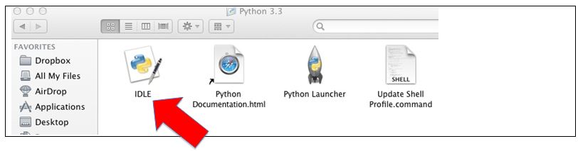 Figure 8.2 Python 3.3
IDLE has the following features:
- coded in 100% pure Python, using the tkinter GUI toolkit
- cross-platform: works mostly the same on Windows, Unix, and Mac OS X
- Python shell window (interactive interpreter) with colorizing of code input, output, and error messages
- multi-window text editor with multiple undo, Python colorizing, smart indent, call tips, auto completion, and other features
- search within any window, replace within editor windows, and search through multiple files (grep)
- debugger with persistent breakpoints, stepping, and viewing of global and local namespaces
configuration, browsers, and other dialogs
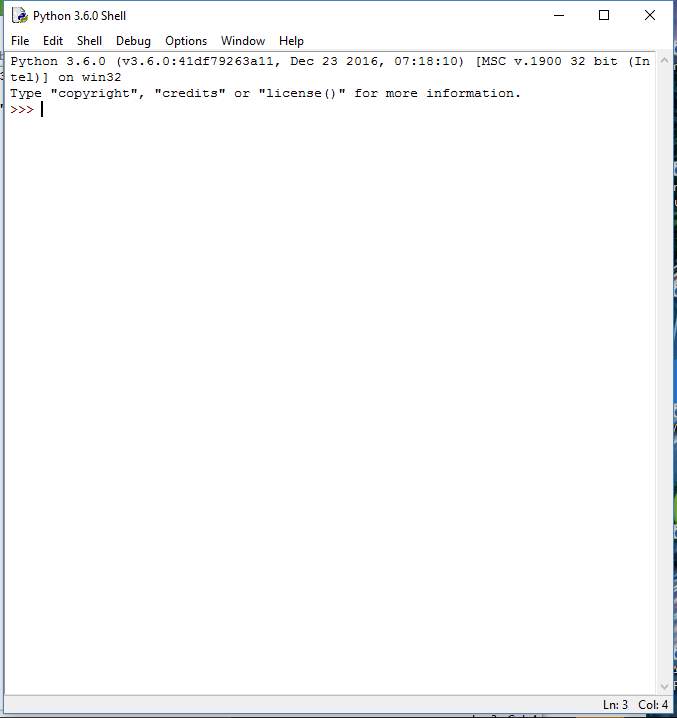
Figure 8.3 Python Shell
8.2 RASPBERRY PI 3:
The Raspberry Pi 3 is the third generation Raspberry Pi. It replaced the Raspberry Pi 2 Model B in February 2016. Compared to the Raspberry Pi 2 it has:
- A 1.2GHz 64-bit quad-core ARMv8 CPU
- 802.11n Wireless LAN
- Bluetooth 4.1
- Bluetooth Low Energy (BLE)
- 1GB RAM
- 4 USB ports
- 40 GPIO pins
- Full HDMI port
- Ethernet port
- Combined 3.5mm audio jack and composite video
- Camera interface (CSI)
- Display interface (DSI)
- Micro SD card slot (now push-pull rather than push-push)
- VideoCore IV 3D graphics core
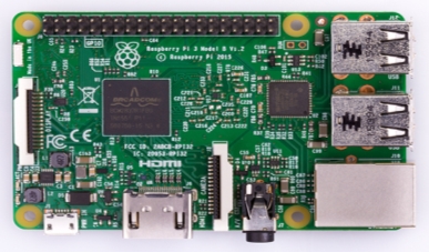
Figure 8.4 Raspberry Pi Model B
The Raspberry Pi 3 has an identical form factor to the previous Pi 2 (and Pi 1 Model B+) and has complete compatibility with Raspberry Pi 1 and 2.
We recommend the Raspberry Pi 3 Model B for use in schools, or for any general use. Those wishing to embed their Pi in a project may prefer the Pi Zero or Model A+, which are more useful for embedded projects, and projects which require very low power.
8.3 Graphical user interface(GUI)
The graphical user interface , is a type of user interface that allows users to interact with electronic devices through graphical icons and visual indicators such as secondary notation, instead of text-based user interfaces, typed command labels or text navigation. GUIs were introduced in reaction to the perceived steep learning curve of command-line interfaces (CLIs), which require commands to be typed on a computer keyboard.
The actions in a GUI are usually performed through direct manipulation of the graphical elements.[Beyond computers, GUIs are used in many handheld mobile devices such as MP3 players, portable media players, gaming devices, smartphones and smaller household, office and industrial controls.
Figure 8.5 GUI
8.4 Proteus Design Suite
The Proteus Design Suite is an Electronic Design Automation (EDA) tool including schematic capture, simulation and PCB Layout modules. It is developed in Yorkshire, England by Labcenter Electronics Ltd with offices in North America and several overseas sales channels. The software runs on the Windows operating system and is available in English, French, Spanish and Chinese languages.
Proteus (PROcessor for TExt Easy to USe) is a fully functional, procedural programming language created in 1998 by Simone Zanella. Proteus incorporates many functions derived from several other languages: C, BASIC, Assembly, Clipper/dBase; it is especially versatile in dealing with strings, having hundreds of dedicated functions; this makes it one of the richest languages for text manipulation.
Its strongest points are:
- powerful string manipulation;
- comprehensibility of Proteus scripts;
- availability of advanced data structures: arrays, queues (single or double), stacks, bit maps, sets, AVL trees.
- The language can be extended by adding user functions written in Proteus or DLLs created in C/C++.
8.4.1 Sequence For execution:
1. Create a new project-
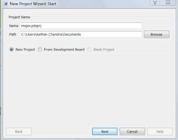
Figure 8.6 Proteus Step1
2. Set a PCB Layout–
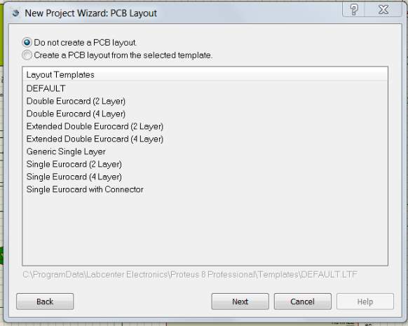
Figure 8.7 Proteus Step2
3. Select the Family as PIC18 and controller as PIC18F87K22
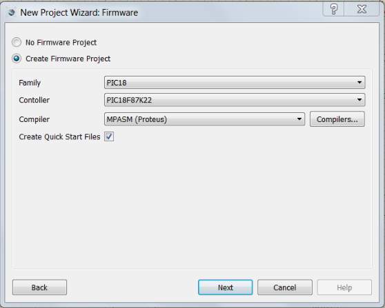
Figure 8.8 proteus Step3
4. Dump the .hex file in the program file box
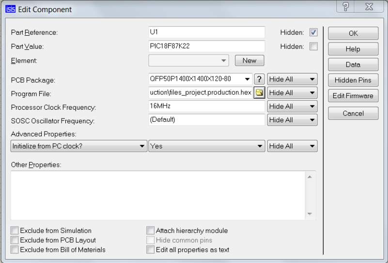
Figure 8.9 Proteus Step 4
8.5 MPLAB IDE
MPLAB IDE is a free, integrated toolset for the development of embedded applications on Microchip’s PIC and dsPIC microcontrollers. It is called an Integrated Development Environment, or IDE, because it provides a single integrated environment to develop code for embedded microcontrollers
Microchip has a large suite of software and hardware development tools integrated within one software package called MPLAB Integrated Development Environment (IDE). MPLAB IDE is a free, integrated toolset for the development of embedded applications on Microchip’s PIC and dsPIC microcontrollers. It is called an Integrated Development Environment, or IDE, because it provides a single integrated environment to develop code for embedded microcontrollers.
8.5.1 Sequence of Steps
1.Open MPLab X IDE
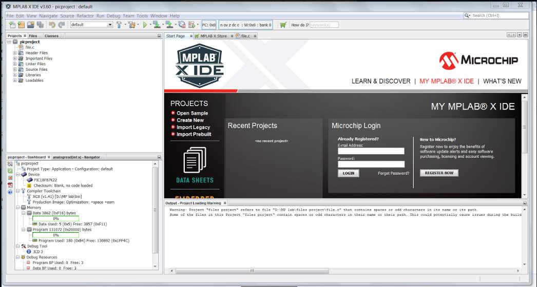
Figure 8.9 MpLab Step 1
2. Create a new project
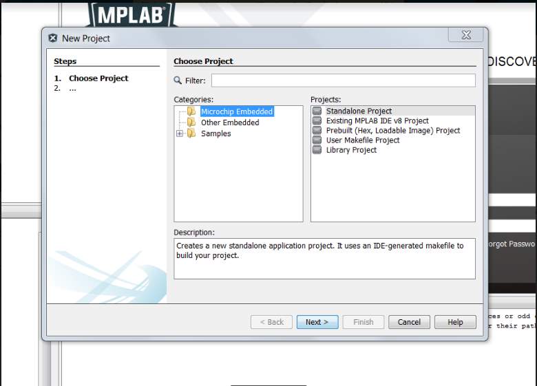
Figure 8.10 MpLab Step 2
3. Select the PIC18 family and select PIC18F87K22 controller
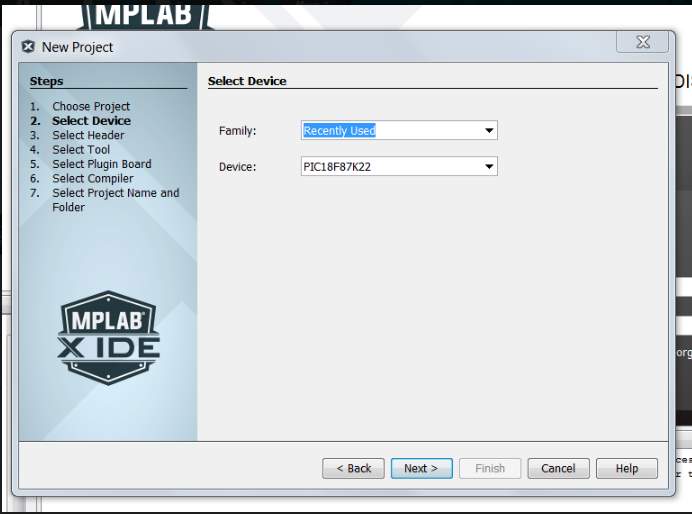
Figure 8.11 MpLab Step 3
4. Select the hardware tools
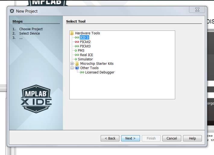
Figure 8.12 MpLab Step 4
5. Select the compiler as XC8
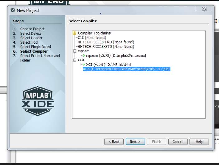
Figure 8.13 MpLab Step 5
6. Create a file and enter the program
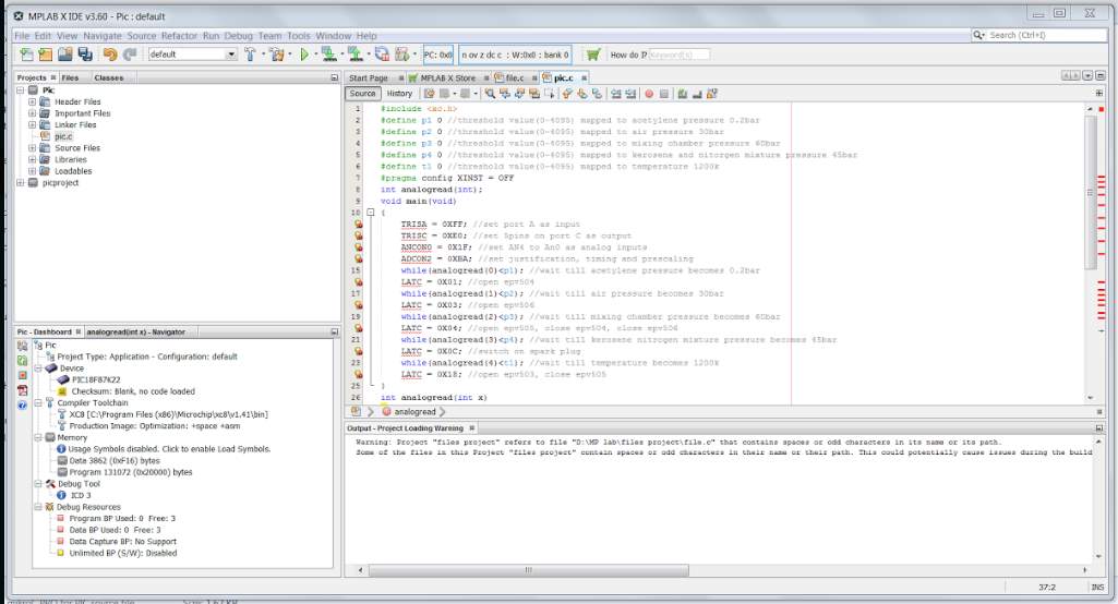
Figure 8.14 MpLab Step 6
7. After entering the program, select run and build the project
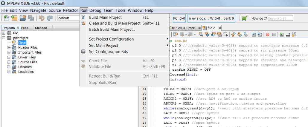
Figure 8.15 MpLab Step 7
8. Check whether the program has no errors
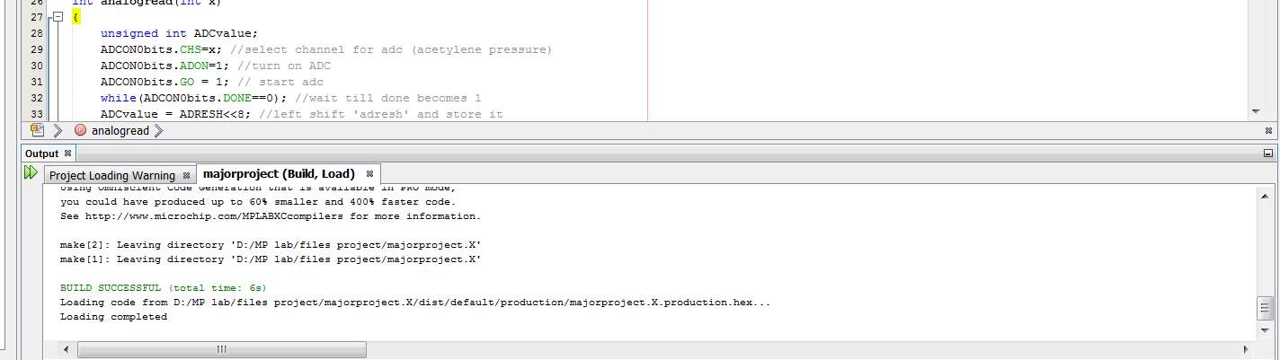
Figure 8.16 MpLab Step 8
MPLAB IDE runs as a 32-bit application on MS Windows, is easy to use and includes a host of free software components for fast application development and super-charged debugging. MPLAB IDE also serves as a single, unified graphical user interface for additional Microchip and third party software and hardware development tools. Moving between tools is a snap, and upgrading from the free software simulator to hardware debug and programming tools is done in a flash because MPLAB IDE has the same user interface for all tools.
8.6 Mikro Program Suite
8.6.1 Sequence of steps
1. Select the PIC18 Family and MCU as PIC18FK22
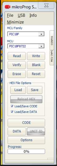
Figure 8.17 Program Suite
2. Select the .hex file and dump it into the PIC18F87K22
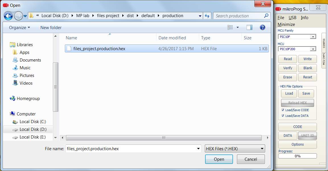
Figure 8.18 Program Suite
8.7 MikroC
8.7.1 Sequences of steps:
1. Create a new project
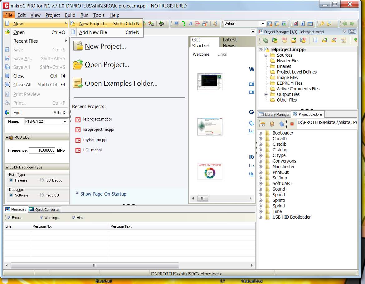
Figure 8.18 Mikroc step 1
2. Select the project type as Standard project
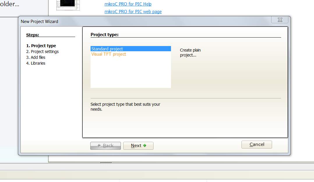
Figure 8.19 Mikroc step2
3. Name the project and select the device as PIC18F87K22 and set device clock at 16MHz.
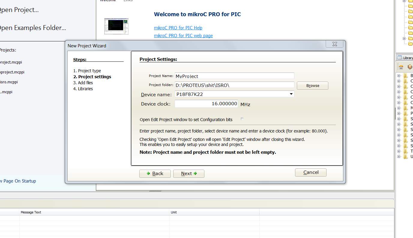
Figure 8.20 Mikroc step3
4. Include all the libraries
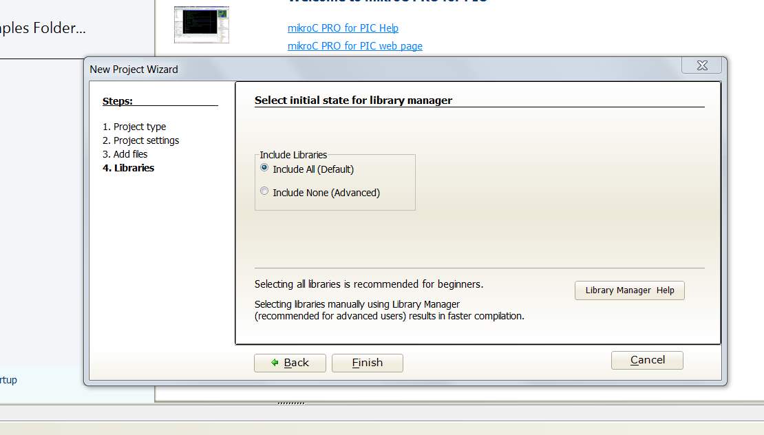
Figure 8.21 Mikroc step4
5. Enter the program and save the file before compiling.
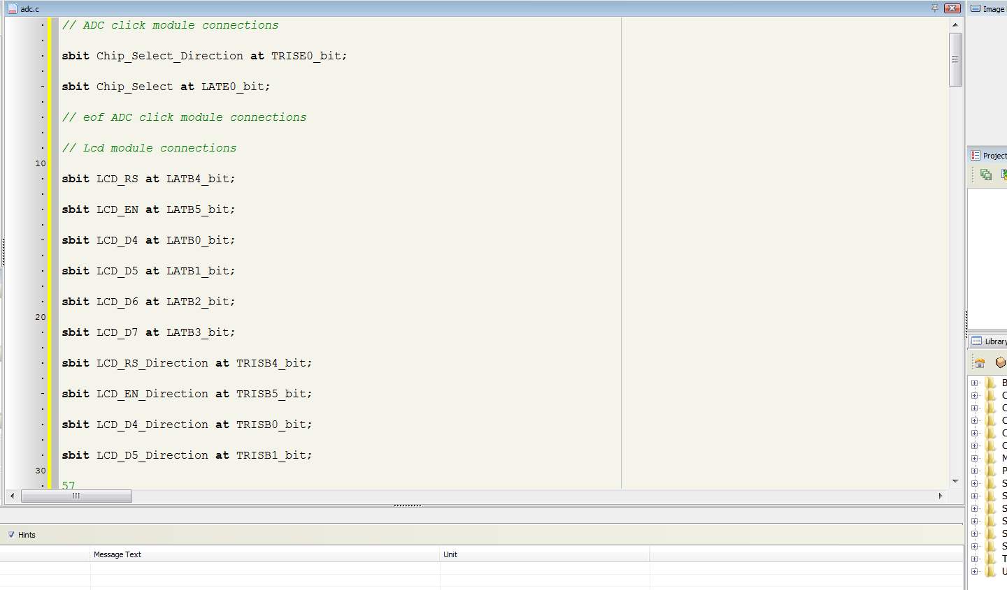
Figure 8.22 Mikroc step 5
6. Then build the program, or use Ctrl+F9
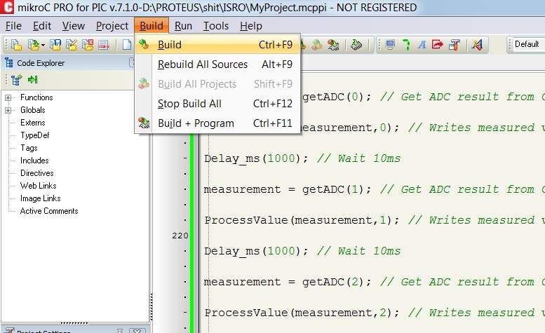
Figure 8.23 Mikroc step 6
7. Check for errors and after check whether the program build is successful.
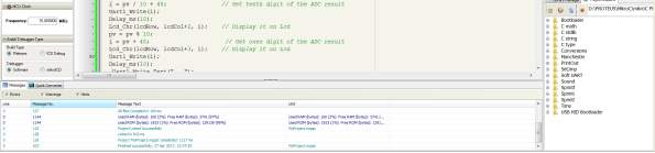
Figure 8.24 Mikroc step 7
CHAPTER 9
SIMULATION AND SYNTHESIS RESULTS
8.1 Proteus Simulation
UART Sender:
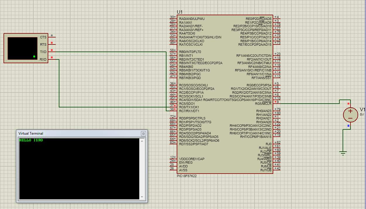
Figure 8.1:UART
UART Sender code:
int i=0;
char uart_rd;
void main() {
Uart1_Init(9600);
Delay_ms(100);
Uart1_Write_Text(“HELLO ISRO”);
uart_rd = ‘sadfgj’;
for(i=0;i<10;i++)
{
UART1_Write(uart_rd);
}
while(1);
}
LCD:
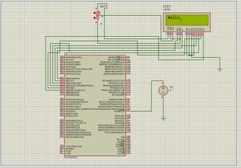
Figure 8.2:LCD
LCD Code:
sbit LCD_RS at RB0_bit;
sbit LCD_EN at RB1_bit;
sbit LCD_D4 at RB2_bit;
sbit LCD_D5 at RB3_bit;
sbit LCD_D6 at RB4_bit;
sbit LCD_D7 at RB5_bit;
sbit LCD_RS_Direction at TRISB0_bit;
sbit LCD_EN_Direction at TRISB1_bit;
sbit LCD_D4_Direction at TRISB2_bit;
sbit LCD_D5_Direction at TRISB3_bit;
sbit LCD_D6_Direction at TRISB4_bit;
sbit LCD_D7_Direction at TRISB5_bit;
void main() {
LCD_Init();
LCD_out(1,1,”Hello”);
}
ADC :
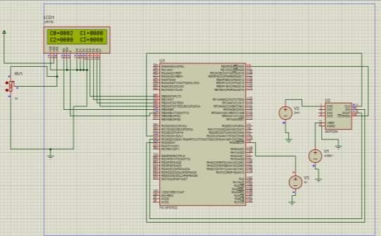
Figure 8.3:ADC
ADC Code:
// ADC click module connections
sbit Chip_Select_Direction at TRISE0_bit;
sbit Chip_Select at LATE0_bit;
// eof ADC click module connections
// Lcd module connections
sbit LCD_RS at LATB4_bit;
sbit LCD_EN at LATB5_bit;
sbit LCD_D4 at LATB0_bit;
sbit LCD_D5 at LATB1_bit;
sbit LCD_D6 at LATB2_bit;
sbit LCD_D7 at LATB3_bit;
sbit LCD_RS_Direction at TRISB4_bit;
sbit LCD_EN_Direction at TRISB5_bit;
sbit LCD_D4_Direction at TRISB0_bit;
sbit LCD_D5_Direction at TRISB1_bit;
sbit LCD_D6_Direction at TRISB2_bit;
sbit LCD_D7_Direction at TRISB3_bit;
// End Lcd module connections
unsigned int measurement, lastValue;
// Get ADC values
unsigned int getADC(unsigned short channel) { // Returns 0..4095
unsigned int tmp;
Chip_Select = 0; // Select MCP3204
SPI1_Write(0x06); // SPI communication using 8-bit segments
channel = channel << 6; // Bits 7 & 6 define ADC input
tmp = SPI1_Read(channel) & 0x0F; // Get first 8 bits of ADC value
tmp = tmp << 8; // Shift ADC value by 8
tmp = tmp | SPI1_Read(0); // Get remaining 4 bits of ADC value
// and form 12-bit ADC value
Chip_Select= 1; // Deselect MCP3204
return tmp; // Returns 12-bit ADC value
}
// Write measured values to Lcd
void processValue(unsigned int pv, unsigned short channel) {
char i, lcdRow, lcdCol;
if (channel < 2) // If ADC channel 0 or 1 is selected
lcdRow = 1; // write in the first Lcd row
else // If ADC channel 2 or is selected
lcdRow = 2; // write in the second Lcd row
if (channel % 2 > 0 ) // If even ADC channel is selected
lcdCol = 13; // select Lcd column 13
else // If odd ADC channel is selected
lcdCol = 4; // select Lcd column 4
// Converting the measured value into 4 characters
// and writing them to the Lcd at the appropriate place
i = pv / 1000 + 48; // Get thousandth digit of the ADC result
Lcd_Chr(lcdRow, lcdCol, i); // Display it on Lcd
pv = pv % 1000;
i = pv / 100 + 48; // Get hundreth digit of the ADC result
Lcd_Chr(lcdRow, lcdCol+1, i); // Display it on Lcd
pv = pv % 100;
i = pv / 10 + 48; // Get tenth digit of the ADC result
Lcd_Chr(lcdRow, lcdCol+2, i); // Display it on Lcd
pv = pv % 10;
i = pv + 48; // Get ones digit of the ADC result
Lcd_Chr(lcdRow, lcdCol+3, i); // Display it on Lcd
}
void main() {
ANCON0 = 0; // Configure ports as digital I/O
ANCON1 = 0;
ANCON2 = 0;
Lcd_Init(); // Initialize Lcd
Lcd_Cmd(_LCD_CLEAR); // Clear display
Lcd_Cmd(_LCD_CURSOR_OFF); // Cursor off
measurement = 0; // Initialize the measurement variable
Chip_Select = 1; // Deselect MCP3204
Chip_Select_Direction = 0; // Set chip select pin to be output
// Initialize SPI1 module at 250kHz, data sampled at the middle of interval
SPI1_Init_Advanced(_SPI_MASTER_OSC_DIV64, _SPI_DATA_SAMPLE_MIDDLE, _SPI_CLK_IDLE_LOW, _SPI_LOW_2_HIGH);
Lcd_Out(1,1,”C0= C1=”); // Display channel 0 and 1 ID on Lcd
Lcd_Out(2,1,”C2= C3=”); // Display channel 2 and 3 ID on Lcd
while (1) {
measurement = getADC(0); // Get ADC result from Channel 0
ProcessValue(measurement,0); // Writes measured value to Lcd
Delay_ms(10); // Wait 10ms
measurement = getADC(1); // Get ADC result from Channel 1
ProcessValue(measurement,1); // Writes measured value to Lcd
Delay_ms(10); // Wait 10ms
measurement = getADC(2); // Get ADC result from Channel 2
ProcessValue(measurement,2); // Writes measured value to Lcd
Delay_ms(10); // Wait 10ms
measurement = getADC(3); // Get ADC result from Channel 3
ProcessValue(measurement,3); // Writes measured value to Lcd
Delay_ms(10); // Wait 10ms
}
}
GLCD:
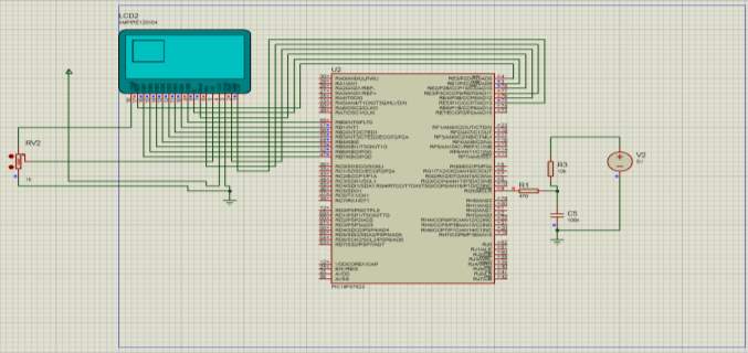
Figure 8.4:GLCD
GLCD Code:
char GLCD_DataPort at PORTD;
sbit GLCD_CS1 at LATC5_bit;
sbit GLCD_CS2 at LATC4_bit;
sbit GLCD_RS at LATC3_bit;
sbit GLCD_RW at LATC2_bit;
sbit GLCD_EN at LATC1_bit;
sbit GLCD_RST at LATC0_bit;
sbit GLCD_CS1_Direction at TRISC5_bit;
sbit GLCD_CS2_Direction at TRISC4_bit;
sbit GLCD_RS_Direction at TRISC3_bit;
sbit GLCD_RW_Direction at TRISC2_bit;
sbit GLCD_EN_Direction at TRISC1_bit;
sbit GLCD_RST_Direction at TRISC0_bit;
void main()
{
glcd_init();
do
{
Glcd_FILL(0xFF);
Delay_ms(1000);
Glcd_FILL(0x00);
Delay_ms(1000);
Glcd_Rectangle(5,5,40,40,1);
Delay_ms(3000);
Glcd_Fill(0x00);
Delay_ms(1000);
Glcd_circle(50,50,10,1);
Delay_ms(1000);
}
while(1);
}
ADC on UART:
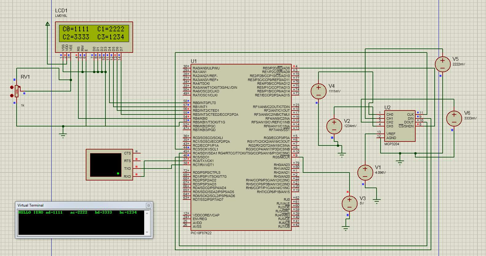
Figure 8.5:ADC on UART
ADC on UART code:
// ADC click module connections
sbit Chip_Select_Direction at TRISE0_bit;
sbit Chip_Select at LATE0_bit;
// eof ADC click module connections
// Lcd module connections
sbit LCD_RS at LATB4_bit;
sbit LCD_EN at LATB5_bit;
sbit LCD_D4 at LATB0_bit;
sbit LCD_D5 at LATB1_bit;
sbit LCD_D6 at LATB2_bit;
sbit LCD_D7 at LATB3_bit;
sbit LCD_RS_Direction at TRISB4_bit;
sbit LCD_EN_Direction at TRISB5_bit;
sbit LCD_D4_Direction at TRISB0_bit;
sbit LCD_D5_Direction at TRISB1_bit;
sbit LCD_D6_Direction at TRISB2_bit;
sbit LCD_D7_Direction at TRISB3_bit;
// End Lcd module connections
unsigned int measurement, lastValue;
// Get ADC values
unsigned int getADC(unsigned short channel) { // Returns 0..4095
unsigned int tmp;
Chip_Select = 0; // Select MCP3204
SPI1_Write(0x06); // SPI communication using 8-bit segments
channel = channel << 6; // Bits 7 & 6 define ADC input
tmp = SPI1_Read(channel) & 0x0F; // Get first 8 bits of ADC value
tmp = tmp << 8; // Shift ADC value by 8
tmp = tmp | SPI1_Read(0); // Get remaining 4 bits of ADC value
// and form 12-bit ADC value
Chip_Select= 1; // Deselect MCP3204
return tmp; // Returns 12-bit ADC value
}
// Write measured values to Lcd
void processValue(unsigned int pv, unsigned short channel) {
char i, lcdRow, lcdCol;
{
if (channel < 2) // If ADC channel 0 or 1 is selected
{lcdRow = 1; // write in the first Lcd row
Uart1_Write_Text(“a”);
}
else // If ADC channel 2 or is selected
{ lcdRow = 2; // write in the second Lcd row
Uart1_Write_Text(“b”);
}
if (channel % 2 > 0 ) // If even ADC channel is selected
{ lcdCol = 13; // select Lcd column 13
Uart1_Write_Text(“c”);
}
else // If odd ADC channel is selected
{lcdCol = 4; // select Lcd column 4
Uart1_Write_Text(“d”);
}
// Converting the measured value into 4 characters
// and writing them to the Lcd at the appropriate place
// Uart1_Write_Text(” measurement “);
//Uart1_Write(j);
Uart1_Write_Text(“=”);
i = pv / 1000 + 48; // Get thousandth digit of the ADC result
Uart1_Write(i);
Delay_ms(10);
Lcd_Chr(lcdRow, lcdCol, i); // Display it on Lcd
pv = pv % 1000;
i = pv / 100 + 48; // Get hundreth digit of the ADC result
Uart1_Write(i);
Delay_ms(10);
Lcd_Chr(lcdRow, lcdCol+1, i); // Display it on Lcd
pv = pv % 100;
i = pv / 10 + 48; // Get tenth digit of the ADC result
Uart1_Write(i);
Delay_ms(10);
Lcd_Chr(lcdRow, lcdCol+2, i); // Display it on Lcd
pv = pv % 10;
i = pv + 48; // Get ones digit of the ADC result
Lcd_Chr(lcdRow, lcdCol+3, i); // Display it on Lcd
Uart1_Write(i);
Delay_ms(10);
Uart1_Write_Text(” “);
}
// if(j==3)
// {j=0;}
}
void main() {
ANCON0 = 0; // Configure ports as digital I/O
ANCON1 = 0;
ANCON2 = 0;
Lcd_Init(); // Initialize Lcd
Uart1_Init(9600);
Delay_ms(100);
Uart1_Write_Text(“HELLO ISRO “);
Lcd_Cmd(_LCD_CLEAR); // Clear display
Lcd_Cmd(_LCD_CURSOR_OFF); // Cursor off
measurement = 0; // Initialize the measurement variable
Chip_Select = 1; // Deselect MCP3204
Chip_Select_Direction = 0; // Set chip select pin to be output
// Initialize SPI1 module at 250kHz, data sampled at the middle of interval
SPI1_Init_Advanced(_SPI_MASTER_OSC_DIV64, _SPI_DATA_SAMPLE_MIDDLE, _SPI_CLK_IDLE_LOW, _SPI_LOW_2_HIGH);
Lcd_Out(1,1,”C0= C1=”); // Display channel 0 and 1 ID on Lcd
Lcd_Out(2,1,”C2= C3=”); // Display channel 2 and 3 ID on Lcd
while (1) {
measurement = getADC(0); // Get ADC result from Channel 0
ProcessValue(measurement,0); // Writes measured value to Lcd
Delay_ms(1000); // Wait 10ms
measurement = getADC(1); // Get ADC result from Channel 1
ProcessValue(measurement,1); // Writes measured value to Lcd
Delay_ms(1000); // Wait 10ms
measurement = getADC(2); // Get ADC result from Channel 2
ProcessValue(measurement,2); // Writes measured value to Lcd
Delay_ms(1000); // Wait 10ms
measurement = getADC(3); // Get ADC result from Channel 3
ProcessValue(measurement,3); // Writes measured value to Lcd
Delay_ms(1000); // Wait 10ms
Uart1_Write_Text(” get: “);
}
}
LM35 :
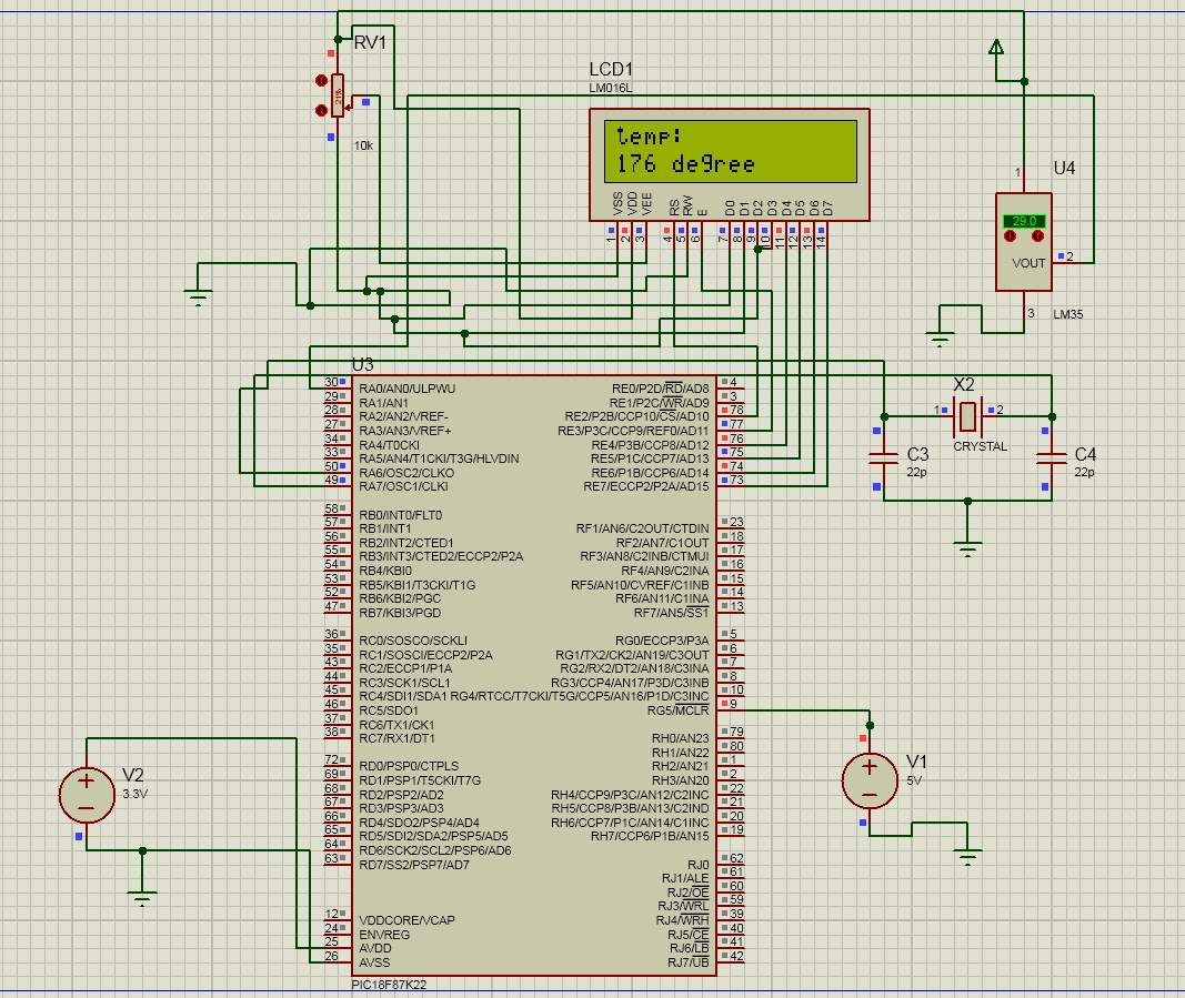
Figure 8.6:LM35
LM35 Code:
sbit LCD_RS at RE2_bit;
sbit LCD_EN at RE3_bit;
sbit LCD_D4 at RE4_bit;
sbit LCD_D5 at RE5_bit;
sbit LCD_D6 at RE6_bit;
sbit LCD_D7 at RE7_bit;
sbit LCD_RS_Direction at TRISE2_bit;
sbit LCD_EN_Direction at TRISE3_bit;
sbit LCD_D4_Direction at TRISE4_bit;
sbit LCD_D5_Direction at TRISE5_bit;
sbit LCD_D6_Direction at TRISE6_bit;
sbit LCD_D7_Direction at TRISE7_bit;
int t;
char b;
char lcd[]=”000 degree”;
void main() {
clc;
ADCON1=0x04;
Lcd_Init();
Lcd_cmd(_LCD_CURSOR_OFF) ;
do
{
Lcd_cmd(_LCD_CLEAR);
Lcd_out(1,1,”temp:”);
t=ADC_Read(0);
t=t*0.4887;
b=t%10;
Lcd[2]=b+’0′;
t=t/10;
b=t%10;
Lcd[1]=b+’0′;
t=t/10;
b=t%10;
Lcd[0]=b+’0′;
Lcd_out(2,1,lcd);
Delay_ms(100);
}while(1);
}
Final Simplified PIC 18F87K22 Code:
#include <xc.h>
#define p1 0 //threshold value(0-4095) mapped to acetylene pressure 0.2bar
#define p2 0 //threshold value(0-4095) mapped to air pressure 30bar
#define p3 0 //threshold value(0-4095) mapped to mixing chamber pressure 60bar
#define p4 0 //threshold value(0-4095) mapped to kerosene and nitorgen mixture pressure 45bar
#define t1 0 //threshold value(0-4095) mapped to temperature 1200k
#pragma config XINST = OFF
int analogread(int);
void main(void)
{
TRISA = 0XFF; //set port A as input
TRISC = 0XE0; //set 5pins on port C as output
ANCON0 = 0X1F; //set AN4 to An0 as analog inputs
ADCON2 = 0XBA; //set justification, timing and prescaling
while(analogread(0)<p1); //wait till acetylene pressure becomes 0.2bar
LATC = 0X01; //open epv504
while(analogread(1)<p2); //wait till air pressure becomes 30bar
LATC = 0X03; //open epv506
while(analogread(2)<p3); //wait till mixing chamber pressure becomes 60bar
LATC = 0X04; //open epv505, close epv504, close epv506
while(analogread(3)<p4); //wait till kerosene nitrogen mixture pressure becomes 45bar
LATC = 0X0C; //switch on spark plug
while(analogread(4)<t1); //wait till temperature becomes 1200k
LATC = 0X18; //open epv503, close epv505
}
int analogread(int x)
{
unsigned int ADCvalue;
ADCON0bits.CHS=x; //select channel for adc (acetylene pressure)
ADCON0bits.ADON=1; //turn on ADC
ADCON0bits.GO = 1; // start adc
while(ADCON0bits.DONE==0); //wait till done becomes 1
ADCvalue = ADRESH<<8; //left shift ‘adresh’ and store it
ADCvalue = ADCvalue|ADRESL; //add adresl value
ADCON0bits.ADON = 0; //turn off adc
return ADCvalue; //send adc value
}
GUI IMAGES:

Figure 8.7:Horizvalve

Figure 8.8:Flame1

Figure 8.9:Flame2

Figure 8.10:Flame2

Figure 8.11:Flame3

Figure 812:Valve

Figure 8.13:Valve1

Figure 8.14:Valve2

Figure 8.15:Sparkn2

Figure 8.16:Sparkn

Figure 8.17:Spark

Figure 8.18:Vertivalve
 Figure 8.19:Picture1
Figure picture2
Figure Picture3
8.2 Python Simulation:
import openpyxl
import matplotlib.pyplot as plt
from tkinter import *
import time
def ign():
while True:
image2 = canvas.create_image(198, 550, anchor=NW, image=filename5)
image2 = canvas.create_image(199, 550, anchor=NW, image=filename1)
tk.update()
time.sleep(0.1)
image2 = canvas.create_image(198, 550, anchor=NW, image=filename5)
image2 = canvas.create_image(199, 550, anchor=NW, image=filename2)
tk.update()
time.sleep(0.1)
image2 = canvas.create_image(198, 550, anchor=NW, image=filename5)
image2 = canvas.create_image(199, 550, anchor=NW, image=filename3)
tk.update()
time.sleep(0.1)
image2 = canvas.create_image(198, 550, anchor=NW, image=filename5)
image2 = canvas.create_image(199, 550, anchor=NW, image=filename4)
tk.update()
time.sleep(0.1)
image2 = canvas.create_image(198,550, anchor=NW, image=filename5)
image2 = canvas.create_image(199, 550, anchor=NW, image=filename3)
tk.update()
time.sleep(0.1)
image2 = canvas.create_image(198, 550, anchor=NW, image=filename5)
image2 = canvas.create_image(199, 550, anchor=NW, image=filename2)
tk.update()
time.sleep(0.1)
def valve1o():
i=0
for i in range(0,10):
image2 = canvas.create_image(247, 69, anchor=NW, image=hv)
image2 = canvas.create_image(242, 80, anchor=NW, image=v1)
tk.update()
time.sleep(0.1)
image2 = canvas.create_image(247, 69, anchor=NW, image=hv)
image2 = canvas.create_image(242, 80, anchor=NW, image=v2)
tk.update()
time.sleep(0.1)
image2 = canvas.create_image(247, 69, anchor=NW, image=hv)
image2 = canvas.create_image(242, 80, anchor=NW, image=v3)
tk.update()
time.sleep(0.1)
i=i+1
image2 = canvas.create_image(247, 69, anchor=NW, image=hv)
image2 = canvas.create_image(242, 80, anchor=NW, image=v1)
def valve2o():
i=0
for i in range(0,10):
image2 = canvas.create_image(247, 158, anchor=NW, image=hv)
image2 = canvas.create_image(242, 169, anchor=NW, image=v1)
tk.update()
time.sleep(0.1)
image2 = canvas.create_image(247, 158, anchor=NW, image=hv)
image2 = canvas.create_image(242, 169, anchor=NW, image=v2)
tk.update()
time.sleep(0.1)
image2 = canvas.create_image(247, 158, anchor=NW, image=hv)
image2 = canvas.create_image(242, 169, anchor=NW, image=v3)
tk.update()
time.sleep(0.1)
i=i+1
image2 = canvas.create_image(247, 158, anchor=NW, image=hv)
image2 = canvas.create_image(242, 169, anchor=NW, image=v1)
def valve3o():
i=0
for i in range(0,10):
image2 = canvas.create_image(347, 239, anchor=NW, image=vv)
image2 = canvas.create_image(351, 234, anchor=NW, image=v1)
tk.update()
time.sleep(0.1)
image2 = canvas.create_image(347, 239, anchor=NW, image=vv)
image2 = canvas.create_image(351, 234, anchor=NW, image=v2)
tk.update()
time.sleep(0.1)
image2 = canvas.create_image(347, 239, anchor=NW, image=vv)
image2 = canvas.create_image(351, 234, anchor=NW, image=v3)
tk.update()
time.sleep(0.1)
i=i+1
image2 = canvas.create_image(347, 239, anchor=NW, image=vv)
image2 = canvas.create_image(351, 234, anchor=NW, image=v1)
def valve4o():
i=0
for i in range(0,10):
image2 = canvas.create_image(470, 287, anchor=NW, image=hv)
image2 = canvas.create_image(465, 298, anchor=NW, image=v1)
tk.update()
time.sleep(0.1)
image2 = canvas.create_image(470, 287, anchor=NW, image=hv)
image2 = canvas.create_image(465, 298, anchor=NW, image=v2)
tk.update()
time.sleep(0.1)
image2 = canvas.create_image(470, 287, anchor=NW, image=hv)
image2 = canvas.create_image(465, 298, anchor=NW, image=v3)
tk.update()
time.sleep(0.1)
i=i+1
image2 = canvas.create_image(470, 287, anchor=NW, image=hv)
image2 = canvas.create_image(465, 298, anchor=NW, image=v1)
def valve1c():
i=0
for i in range(0,10):
image2 = canvas.create_image(247, 69, anchor=NW, image=hv)
image2 = canvas.create_image(242, 80, anchor=NW, image=v1)
tk.update()
time.sleep(0.1)
image2 = canvas.create_image(247, 69, anchor=NW, image=hv)
image2 = canvas.create_image(242, 80, anchor=NW, image=v3)
tk.update()
time.sleep(0.1)
image2 = canvas.create_image(247, 69, anchor=NW, image=hv)
image2 = canvas.create_image(242, 80, anchor=NW, image=v2)
tk.update()
time.sleep(0.1)
i=i+1
image2 = canvas.create_image(247, 69, anchor=NW, image=hv)
image2 = canvas.create_image(242, 80, anchor=NW, image=v1)
def valve2c():
i=0
for i in range(0,10):
image2 = canvas.create_image(247, 158, anchor=NW, image=hv)
image2 = canvas.create_image(242, 169, anchor=NW, image=v1)
tk.update()
time.sleep(0.1)
image2 = canvas.create_image(247, 158, anchor=NW, image=hv)
image2 = canvas.create_image(242, 169, anchor=NW, image=v3)
tk.update()
time.sleep(0.1)
image2 = canvas.create_image(247, 158, anchor=NW, image=hv)
image2 = canvas.create_image(242, 169, anchor=NW, image=v2)
tk.update()
time.sleep(0.1)
i=i+1
image2 = canvas.create_image(247, 158, anchor=NW, image=hv)
image2 = canvas.create_image(242, 169, anchor=NW, image=v1)
def valve3c():
i=0
for i in range(0,10):
image2 = canvas.create_image(347, 239, anchor=NW, image=vv)
image2 = canvas.create_image(351, 234, anchor=NW, image=v1)
tk.update()
time.sleep(0.1)
image2 = canvas.create_image(347, 239, anchor=NW, image=vv)
image2 = canvas.create_image(351, 234, anchor=NW, image=v3)
tk.update()
time.sleep(0.1)
image2 = canvas.create_image(347, 239, anchor=NW, image=vv)
image2 = canvas.create_image(351, 234, anchor=NW, image=v2)
tk.update()
time.sleep(0.1)
i=i+1
image2 = canvas.create_image(347, 239, anchor=NW, image=vv)
image2 = canvas.create_image(351, 234, anchor=NW, image=v1)
def spark():
i=0
time.sleep(1)
canvas.itemconfig(vs, fill=”#00ff00″)
tk.update()
for i in range(0,10):
image2 = canvas.create_image(374, 338, anchor=NW, image=sp)
tk.update()
time.sleep(0.1)
image2 = canvas.create_image(374, 338, anchor=NW, image=sn)
tk.update()
time.sleep(0.1)
i=i+1
canvas.itemconfig(vs, fill=”#ff0000″)
image2 = canvas.create_image(374, 338, anchor=NW, image=sn2)
tk.update()
def mix():
i=0
z=””
x=255
y=255
for i in range(0,21):
time.sleep(0.1)
x=x-4
y=y-8
z=’#’+ hex(x)[2:4]+ hex(y)[2:4]+ hex(y)[2:4]
canvas.itemconfig(mc, fill=z)
tk.update()
def gas():
i=0
z=””
x=255
y=255
for i in range(0,21):
time.sleep(0.1)
x=x-4
y=y-8
z=’#’+ hex(x)[2:4]+ hex(y)[2:4]+ hex(y)[2:4]
canvas.itemconfig(gc, fill=z)
tk.update()
tk=Tk()
canvas = Canvas(tk, width=766, height=767)
tk.title(“ILLUSTRATION”)
canvas.pack()
p1 = canvas.create_rectangle(62, 13, 109, 59, fill=”#ff0000″)
p2 = canvas.create_rectangle(62, 242, 109, 286, fill=”#ff0000″)
p3 = canvas.create_rectangle(354, 13, 409, 59, fill=”#ff0000″)
p4 = canvas.create_rectangle(513, 13, 565, 59, fill=”#ff0000″)
ac = canvas.create_rectangle(18, 66, 256, 142, fill=”#ff5050″)
ai = canvas.create_rectangle(18, 156, 256, 236, fill=”#606060″)
mc = canvas.create_rectangle(270, 66, 442, 248, fill=”#ffffff”)
kc = canvas.create_rectangle(501, 66, 575, 335, fill=”#79cee3″)
gc = canvas.create_rectangle(113, 268, 491, 567, fill=”#ffffff”)
vs = canvas.create_rectangle(582, 332, 733, 411, fill=”#ff0000″)
t1 = canvas.create_rectangle(290, 235, 333, 276, fill=”#ff0000″)
filename = PhotoImage(file = “Picture1.png”)
image = canvas.create_image(0,0, anchor=NW, image=filename)
filename1 = PhotoImage(file = “flame1.png”)
filename2 = PhotoImage(file = “flame2.png”)
filename3 = PhotoImage(file = “flame3.png”)
filename4 = PhotoImage(file = “flame4.png”)
filename5 = PhotoImage(file = “none.png”)
hv = PhotoImage(file = “horizvalve.png”)
vv = PhotoImage(file = “vertivalve.png”)
v1 = PhotoImage(file = “valve.png”)
v2 = PhotoImage(file = “valve1.png”)
v3 = PhotoImage(file = “valve2.png”)
sp = PhotoImage(file = “spark.png”)
sn = PhotoImage(file = “sparkn.png”)
sn2 = PhotoImage(file = “sparkn2.png”)
image2 = canvas.create_image(247, 69, anchor=NW, image=hv)
image2 = canvas.create_image(247, 158, anchor=NW, image=hv)
image2 = canvas.create_image(347, 239, anchor=NW, image=vv)
image2 = canvas.create_image(470, 287, anchor=NW, image=hv)
image2 = canvas.create_image(242, 80, anchor=NW, image=v1)
image2 = canvas.create_image(242, 169, anchor=NW, image=v1)
image2 = canvas.create_image(351, 234, anchor=NW, image=v1)
image2 = canvas.create_image(465, 298, anchor=NW, image=v1)
time.sleep(1)
canvas.itemconfig(p1, fill=”#00ff00″)
tk.update()
valve1o()
time.sleep(1)
canvas.itemconfig(p2, fill=”#00ff00″)
tk.update()
valve2o()
mix()
canvas.itemconfig(p3, fill=”#00ff00″)
tk.update()
valve1c()
valve2c()
valve3o()
gas()
canvas.itemconfig(p4, fill=”#00ff00″)
tk.update()
spark()
canvas.itemconfig(gc, fill=”#ffc90e”)
tk.update()
canvas.itemconfig(t1, fill=”#00ff00″)
tk.update()
valve3c()
valve4o()
ign()

Figure8.20 Python Logo
8.3 Final PIC assembly code
#include <xc.h>
#define p1 0 //threshold value(0-4095) mapped to acetylene pressure 0.2bar
#define p2 0 //threshold value(0-4095) mapped to air pressure 30bar
#define p3 0 //threshold value(0-4095) mapped to mixing chamber pressure 60bar
#define p4 0 //threshold value(0-4095) mapped to kerosene and nitorgen mixture pressure 45bar
#define t1 0 //threshold value(0-4095) mapped to temperature 1200k
#pragma config XINST = OFF
int analogread(int);
void main(void)
{
TRISA = 0XFF; //set port A as input
TRISC = 0XE0; //set 5pins on port C as output
ANCON0 = 0X1F; //set AN4 to An0 as analog inputs
ADCON2 = 0XBA; //set justification, timing and prescaling
while(analogread(0)<p1); //wait till acetylene pressure becomes 0.2bar
LATC = 0X01; //open epv504
while(analogread(1)<p2); //wait till air pressure becomes 30bar
LATC = 0X03; //open epv506
while(analogread(2)<p3); //wait till mixing chamber pressure becomes 60bar
LATC = 0X04; //open epv505, close epv504, close epv506
while(analogread(3)<p4); //wait till kerosene nitrogen mixture pressure becomes 45bar
LATC = 0X0C; //switch on spark plug
while(analogread(4)<t1); //wait till temperature becomes 1200k
LATC = 0X18; //open epv503, close epv505
}
int analogread(int x)
{
unsigned int ADCvalue;
ADCON0bits.CHS=x; //select channel for adc (acetylene pressure)
ADCON0bits.ADON=1; //turn on ADC
ADCON0bits.GO = 1; // start adc
while(ADCON0bits.DONE==0); //wait till done becomes 1
ADCvalue = ADRESH<<8; //left shift ‘adresh’ and store it
ADCvalue = ADCvalue|ADRESL; //add adresl value
ADCON0bits.ADON = 0; //turn off adc
return ADCvalue; //send adc value
}
CHAPTER 9
CONCLUSION
The main objectives of this project condensed down to three are
- The cold flow and hot flow tests results will be useful in comparing and arriving at a reasonable estimate for the actual scale of GSLV-M3 during lift-off.
- Reduced attenuation levels mainly in terms of acoustics.
- To maintain a constant Mach number by varying stagnation temperatures.
A remote operation of the varied transducers, sensors, valves and other components makes it more practical. The project can be up scaled to be used in a PLC which is used in the actual model of the gas generator. The relays are easily manoeuvrable and the sequence is easily manipulated as python provides for number of options and the PIC microcontroller can be reprogrammed without any hassle.
Subsequently the study is carried out to investigate the effect of different Mixture ratios and other conditions required during lift off
9.1 Future Scope
The first test-flight of the GSLV with a cryogenic upper, or third, stage happened in April 2001. It was a failure. After that, eight flights of the rocket have happened over the next 14 years. Of these, five flew with a Russian cryogenic engine onboard while the other three used the indigenously developed ones. Three succeeded, four failed and one was a partial success. The first successful test-flight using the Russian engine happened in May 2003. The first successful test-flight using the indigenous engine happened in January 2014. The Mk-II uses four liquid-fuel strap-on boosters in addition to the first stage and the CE-7.5 indigenous cryogenic engine for the third. The Mk-III will use two solid-fuel boosters for the first stage and the CE-20 indigenous cryogenic engine for the third. It will also carry the 3.2-ton GSAT 19 satellite. A flight in December 2014 had only two functional stages – the CE-20 engine to be used on it had been under development. This engine produces a nominal thrust of 200 kN, but has an operating thrust range between 180 kN to 220 kN and can be set to any fixed values between them. The engine is first of its kind that works in gas generator cycle and indigenously developed. Thus by eliminating the use of solid fuel and using cryogenic liquids and gases the payload of the launch vehicle can be reduced.
CHAPTER 10
REFERENCES
- Huzel.D.K and Huang.G.H, 1992 Modern Engineering for Design of Liquid Propellant Rocket Engines (American Institute of Aeronautics and Astronautics
- Sutton,G.P, 1992, Rocket Propulsion Elements : An introduction to the Engineering of Rockets (John Wiley & sons, Inc)
- White F.M, 1979 Fluid Mechanics (McGraw-Hill Book Company 1979)
- Gordon.s and MCBride, B.J, 1971 “ Computer Program for calculation of Complex Chemical Equilibrium Compositions, Rocket Performance, Incident and Reflection shocks and Chapman-Jougent Detonations”, NASA SP-273.
- Numerical investigation of thermal stratification in cryogenic tanks subjected to wall heat flux, NASA TM 103/94, AIAA-90-2375
- Eckert, E. R. G and Jackson, T. W, “Analysis of turbulent free convection boundary layer on a flat plate;” NACA Rept, 1015 (July 12, 1950).
- Bailey T, Vandekoppel,R and Skartvedt, G “Cryogenic Propellant stratification and test correlation” AIAA JI, 1657-1659 (1963)
- Schmidt, A, Purcell, J, Wilson, W A, and Smith, R, “An experimental study concerning the pressurization and stratification of liquid hydrogen”, Advances in Cryogenic Engg 5, 487-497 (1960).
- Huntley, S C “Temperature pressure-time relations in a closed container,” NACA TN 4259 (1958).
- Neff, R “A survey of stratification in a cryogenic liquid” Advances in Cryogenic Engg 5, 460-466 (1960)
- Richards, H, and Merrill, H, “Analytical and experimental determination of liquid hydrogen stratification,” Final Rept, Martin Marietta Corp, Denver, Colo, Control TP2 83504 (April 1963).
- Lin C S, Hasan M M, 1990 Numerical Investigation of The Thermal Stratification in Cryogenic Tanks Subjected to Wall Heat Flux, AIAA-90-2375, NASA Tech. Memo. 103194
- Barsi S, and Kassemi M, 2008, Numerical and Experimental Comparisons of the Self pressurization behavior of an LH2 tank in Normal Gravity, Cryogenics Vol. 48, pp. 122-129.
- Behnel S 2008 The Cython compiler for C-extensions in Python Proc. of EuroPython-08 (Vilnius/Lietuva, 2008) Bronevetsky G, Marques D, Pingali K and Stodghill P 2003 Automated application-level checkpointing of MPI programs PPoPP ’03: Proc. 9th ACM SIGPLAN Symp. on Principles and Practice of Parallel Programming (New York, NY, USA: ACM Press) pp 84–94
- Python Team 2014 Pdb—the Python debugger (accessed July 2014)
- Python Team 2014 Pickle—Python object serialization (accessed July 2014)
- http://download.mikroe.com/documents/standards/mikrobus/mikrobus-standard-specification-v200.pdf
- http://ww1.microchip.com/downloads/en/DeviceDoc/39960d.pdf
- http://download.mikroe.com/documents/add-on-boards/click/adc/adc-click-manual-v100.pdf
- https://en.wikipedia.org/wiki/Geosynchronous_Satellite_Launch_Vehicle_Mark_III
- http://www.shar.gov.in/SDSCE/index.jsp
- http://www.diva-portal.se/smash/get/diva2:708570/FULLTEXT01.pdf
- http://www.pyromation.com/Downloads/Doc/Training_TC_Theory.pdf
- http://www.pyromation.com/Downloads/Data/emfk_c.pdf
- https://en.wikipedia.org/wiki/Electro-pneumatic_action
- http://nptel.ac.in/courses/112106175/Module%204/Lecture%2041.pdf
- http://ieeexplore.ieee.org/document/5448483/
- http://www.ijcna.org/Manuscripts/Volume-2/Issue-1/Vol-2-issue-1-M-04.pdf
- (http://behnel.de/cythonEP2008/cython-ep2008.html)
ANNEXURE – I
Temperature values for different mixture ratios (air/kerosene) is listed below,
| Mixture Ratio (Air/Kerosene)
(MR) |
Temperature
(in K) |
| 9 | 1665 |
| 10 | 1782 |
| 11 | 1883 |
| 13 | 2049 |
| 15 | 2179 |
| 17 | 2161 |
| 19 | 2012 |
| 21 | 1883 |
| 23 | 1772 |
| 25 | 1676 |
| 27 | 1592 |
| 29 | 1518 |
| 31 | 1452 |
| 33 | 1393 |
| 35 | 1340 |
| 37 | 1292 |
| 39 | 1248 |
| 41 | 1208 |
Cite This Work
To export a reference to this article please select a referencing stye below:
Related Services
View all


Related Content
All TagsContent relating to: "Energy"
Energy regards the power derived from a fuel source such as electricity or gas that can do work such as provide light or heat. Energy sources can be non-renewable such as fossil fuels or nuclear, or renewable such as solar, wind, hydro or geothermal. Renewable energies are also known as green energy with reference to the environmental benefits they provide.
Related Articles

DMCA / Removal Request
If you are the original writer of this dissertation and no longer wish to have your work published on the UKDiss.com website then please: