Effects of Severe Icing Conditions on Aerodynamic Performance of Cessna 152 Aircraft
Info: 26568 words (106 pages) Dissertation
Published: 13th Dec 2019
Tagged: Environmental StudiesAviation
EFFECTS OF SEVERE ICING CONDITIONS ON AERODYNAMIC PERFORMANCE OF CESSNA 152 AIRCRAFT
ABSTRACT
The accretion of ice on an aircraft is dangerous to flight safety. Icing on a wing of an aircraft can significantly reduce the aerodynamic performance. There are different types of icing conditions resulting in different ice accretions. Hence, evaluation of the process and outcomes of ice accretion is vital to ensure safety. In this project, the adverse effects of ice accretion on aircraft are studied. The icing effects are examined using experimental, numerical and theoretical methods. A brief comparison between the results, achieved by comparing the three methods, of this project with the published data, suggest that the findings of this study are valid and useful.
TABLE OF CONTENTS
2.5 Similar Wind Tunnel Experiments
2.6 Similar Numerical Simulation
3.1.1 Theoretical Lift Coefficient
3.1.2 Theoretical Drag Coefficient
5.1.3 Physics Models and Boundary Condition
6.1.1 Bare Wing Comparison of the Three Methods
6.2 Effects of Clear, Rime and Mixed Ice
6.2.1 CFD Comparison of Effects of Ice
6.2.2 Further Analysis and Recommendation
APPENDIX B – NACA 0012 Aerofoil Coordinates
APPENDIX C – EXPERIMENTAL RESULTS FOR BARE WING
APPENDIX D – RIME ICE EXPERIMENTAL RESULTS
APPENDIX E – CLEAR ICE EXPERIMENTAL RESULTS
APPENDIX F – MIXED ICE EXPERIMENTAL RESULTS
APPENDIX G – CFD BENCHMARK LIFT AND DRAG COEFFICIENT PLOTS
APPENDIX I – CFD PLOTS FOR ICED WING
APPENDIX J – THEORETICAL AND EXPERIMENTAL COMPARISON GRAPHS FOR BARE WING
LIST OF FIGURES
Figure 1 Different Types of Structural Icing on Aircraft’s Wing (Chapter 10 – ICING, 2017)
Figure 2 NACA 0012 Aerofoil (“NACA 0012 AIRFOILS (N0012-Il)”)
Figure 3 CATIA Model of the Wing
Figure 5 Wing Development at Different Stages
Figure 7 Open Return Wind Tunnel
Figure 8 Geometrical Setup in Star CCM+
Figure 10 Volume Mesh around the Wing
Figure 11 Velocity Contour Plot for α = 0°
Figure 13 Flow Visualisation around Bare Wing (AOA 10)
Figure 14 Flow Visualisation around Iced Wing (AOA 10)
Figure 15 Screenshot of XFOIL Command Window
Figure 16 CL Plot for CFD Benchmark Test (AOA 10)
Figure 17 CD Plot for CFD Benchmark Test (AOA 10)
Figure 18 Residual for Bare Wing simulation AOA of 0
Figure 19 CL Plot for Bare Wing simulation AOA of 0
Figure 20 CD Plot for Bare Wing simulation AOA of 0
Figure 21 Residual for Bare Wing simulation AOA of -4
Figure 22 CL Plot for Bare Wing simulation AOA of -4
Figure 23 CD Plot for Bare Wing simulation AOA of -4
Figure 24 Residual for Bare Wing simulation AOA of 10
Figure 25 CL Plot for Bare Wing simulation AOA of 10
Figure 26 CD Plot for Bare Wing simulation AOA of 10
Figure 27 Residual for Clear Iced Wing simulation, AOA of -4
Figure 28 CL Plot for Clear Iced Wing simulation, AOA of -4
Figure 29 CD Plot for Clear Iced Wing simulation, AOA of -4
Figure 30 Residual for Clear Iced Wing simulation, AOA of 10
Figure 31 CL Plot for Clear Iced Wing simulation, AOA of 10
Figure 32 CD Plot for Clear Iced Wing simulation, AOA of 10
Figure 33 Theoretical and Experimental Comparison Re 250000
Figure 34 Theoretical and Experimental Comparison Re 300000
Table 1 2D Lift Coefficient for 200000 Reynold’s Number
Table 2 Theoretical Lift Coefficient
Table 3 Skin Friction Drag from XFOIL
Table 4 Theoretical Drag Coefficient for Reynolds Number of 200000
Table 5 Theoretical Lift and Drag Coefficients for Re 250000
Table 6 Theoretical Lift and Drag Coefficients for Re 300000
Table 7 Properties of Different Modelling Materials
Table 8 Wind Tunnel Data for Re 200000
Table 9 Experimental Results for Bare Wing
Table 10 Experimental Results for Rime Ice
Table 11 Experimental Results for Clear Ice
Table 12 Experimental Results for Mixed Ice
Table 13 Theoretical and Numerical Benchmark Comparison
Table 14 CFD Results (Bare Wing)
Table 15 CFD Results (Clear Iced Wing)
Table 16 Bare Wing Comparison for RE 300000
Table 17 Clear Iced Wing comparison between Numerical and Experimental Results
Table 18 Wind Tunnel Data for RE 250000 (Bare Wing)
Table 19 Wind Tunnel Data for RE 300000 (Bare Wing)
Table 20 Wind Tunnel Data for RE 200000 (Rime Iced Wing)
Table 21 Wind Tunnel Data for RE 250000 (Rime Iced Wing)
Table 22 Wind Tunnel Data for RE 300000 (Rime Iced Wing)
Table 23 Wind Tunnel Data for RE 200000 (Clear Iced Wing)
Table 24 Wind Tunnel Data for RE 250000 (Clear Iced Wing)
Table 25 Wind Tunnel Data for RE 300000 (Clear Iced Wing)
Table 26 Wind Tunnel Data for RE 200000 (Mixed Iced Wing)
Table 27 Wind Tunnel Data for RE 250000 (Mixed Iced Wing)
Table 28 Wind Tunnel Data for RE 300000 (Mixed Iced Wing)
Graph 5‑1 Residuals of Benchmark Test
Graph 5‑2 Pressure Distribution across the NACA 0012 Aerofoil
Graph 6‑1 Bare Wing Lift Comparison for Re 200000
Graph 6‑2 Bare Wing Drag Comparison for Re 200000
Graph 6‑3 Comparison of Lift for different Ice Simulations (RE 200000)
Graph 6‑4 Comparison of Drag for different Ice Simulations (RE 200000)
Graph 6‑5 Comparison of Lift for different Ice Simulations (RE 250000)
Graph 6‑6 Comparison of Drag for different Ice Simulations (RE 250000)
Graph 6‑7 Comparison of Lift for different Ice Simulations (RE 300000)
Graph 6‑8 Comparison of Drag for different Ice Simulations (RE 300000)
Graph 6‑9 Comparison of Surface Pressure Distribution Between Iced and Bare Wing
GLOSSARY
CL
3D Lift Coefficient
Cl
2D Lift Coefficient
L
Lift Force
D
Drag Force
CD
Drag Coefficient
CDo
Parasitic/Skin-Friction Drag Coefficient of an Aerofoil
CDi
Induced Drag Coefficient
Cp
Pressure Coefficient
α
Angle of Attack (AOA)
AR Aspect Ratio of a Wing
b
Span of a wing
S
Wing Planform/Reference Area
RE Reynolds Number
e
Oswald Efficiency factor of a Wing
ρ
Density of air
v
Velocity of air
CFD Computational Fluid Dynamics
1 INTRODUCTION
Aerodynamics is a study of airflow around an aircraft when it flies at a given velocity. There are four major forces acting on aircraft lift, drag, weight and thrust. The weight of an aircraft is the force due to gravity. The weight of an aircraft determines the amount of lift needed. Lift is an upward force and it must be greater than the weight which allows an aircraft to fly. Drag is type of friction force, acting opposite to the direction of the aircraft, which causes resistance around its surface; reducing its velocity. The prime focus will be on lift and drag for the project as I will be analysing just the wing of the aircraft. The reason being that the wing plays a major role in aircraft aerodynamics and it produces the most amount of lift and drag of an aircraft.
Flying is the most common and by far the safest mode of travel today. However, there are lot of safety measures and factors that need to be considered for an aircraft to be safe for a flight. Weather is one of the most important of these factors. Hence, it needs a lot of consideration. There are many different weather conditions that affect an aircraft in different ways. Some conditions are ideal for aircraft performance whereas some are not, different weather conditions have different effect on the aerodynamic performance of an aircraft.
1.1 Aims
To provide an overview of adverse effects of ice formation on Cessna 152 aircraft and to investigate the various impacts on the aerodynamic factors of the aircraft.
1.2 Objectives
- Literature Review: Brief research on various unfavourable weather conditions and their effects on aircraft performance, with detailed investigation on icing effects including any tests that have been undertaken to investigate its impact.
- Experiment: Testing of an aerofoil, with and without ice formation, using a wind tunnel and obtain aerodynamic results such as coefficient of lift and drag.
- Calculations: Undertake various aerodynamic calculations such as lift, drag and lift-to-drag ratio at different conditions. This includes both the theoretical and experimental calculations.
- Computational Fluid Dynamics (CFD): Perform a brief flow investigation over an aerofoil using advanced CFD software and then compare that with theoretical and experimental results.
- Analysis: Comparison of obtained results from calculations and experiment and to analyse them to draw a conclusion, including the comparison of theoretical, experimental and numerical results.
1.3 Summary
In this project, the main focus was on the effects of severe icing conditions on aerodynamic performance of Cessna 152 aircraft. An in-depth investigation on the causes and effects of severe icing conditions and how they impact the flight of an aircraft was undertaken. Light aircrafts, like the Cessna 152, are specifically vulnerable to such conditions as they are not equipped with latest safety technologies available in most modern aircrafts. This study includes wind tunnel testing to obtain experimental results which are compared with theoretical and numerical results to understand the effects of ice in more detail.
The model of the aerofoil used in the Cessna 152 was used to investigate the effects of ice on the aerodynamic properties. Since, the wing plays a major role in the aerodynamics of an aircraft, it is important to evaluate these effects. It is difficult to produce the model of the whole aircraft and so a model of the wing is developed. The Cessna 152 uses two different aerofoils in its wings. NACA 2412 at the root and NACA 0012 at the tip of the wing. After consulting the technicians and due consideration, it was concluded that a constant shape throughout the span of the model is assumed, purely to reduce the complexity of the model and to save time. Hence, NACA 0012 was used as the aerofoil for this project and the wing was developed based on this.
The effects of Icing are emphasised in this project. The reason by behind ice accretion is discussed, including where it formed. A detailed evaluation is undertaken for different types of ice accretions and their properties that are affecting the aircraft’s aerodynamic performance.
2 LITERATURE REVIEW
2.1 Background of Aircraft
The aircraft that I will focusing in this study is the Cessna 152. The Cessna 152 came into production in 1978 and it was revised model of its predecessor the Cessna 152. The Cessna 152 is two seater light aircraft with a payload of 1670 pounds. It has tricycle landing gear and a 110-horsepower Lycoming O-235 engine. The Cessna 152 was fuel efficient when compared to predecessor and therefore it was highly successful aircraft of its time. Due to it being light in nature, it was widely used by many commercial pilots and trainers. The Cessna 152 went off production in 1985. It is still widely used to train students and is a highly cost effective starter aircraft (Disciples of Flight, 2017).
2.2 Favourable Conditions
There are some conditions which are said to be ideal for an aircraft as this when the aircraft performance is at its best. These include clear skies and still air where the wing can produce lift more efficiently during take-off. These conditions also include ideal density, temperature, pressure and wind where the aircraft can easily stabilize itself during the flight. The lack of wind would mean there would be no turbulence during flight which would ensure efficient performance of the aircraft. However, in the real world, the weather changes and is not always so obliging. Hence, we need to consider different adverse conditions which are listed below.
2.3 Unfavourable Conditions
There are many weather conditions which are unsuitable for aircraft performance. Some of which are listed below:
- Extreme icing conditions: The most adverse weather condition for aircraft performance is the extreme icing. The build of ice before or during the flight can drastically change the aerodynamic performance of an aircraft. Icing conditions occur when the temperature outside is below the freezing point which causes the atmospheric moisture to create ice, which then effects the overall aircraft performance. “Aircraft with low wing loadings have relatively large surface areas. For such aircraft, an accumulation of 6 to 12 mm ice or snow can represent a significant increase in aircraft weight” (Smetana, 2001). This shows even a small build of ice on an aircraft has a huge impact on its performance. Icing is hazardous to an aircraft in many ways. For example, icing on control surfaces and wings reduces lift produced as overall weight of the aircraft increases, generates inaccurate instrument readings and compromises flight control. Build of small ice particles in the engine reduces performance which leads to reduction of power generated affecting the overall efficiency of the aircraft.
- Extreme Heat: Very high temperatures reduce the air density significantly which is very dangerous for aircraft performance as density is a major factor that affects aerodynamics. The aerodynamic performance of an aircraft decreases when air density decreases as that is when the air molecules are further away from each other, hence decreased air density. The performance of your airplane relies on the air thickness: which directly affects lift, drag, engine performance and thrust. Consequently, you can say that when air thickness reduces, aerodynamic performance likewise reduces. In this case, the indicated airspeed of an aircraft remains the same during take-off. However, since the air density is reduced, true air speed is higher and so is the ground speed. Therefore, to achieve the indicated air speed, longer distance is required for take-off and because the engine thrust is lower, take-off speed requires more time which means longer runway is needed to achieve this.
- Wind Shear: “Wind shear is a change in wind speed and/or direction over a short distance. It can occur either horizontally or vertically and is most often associated with strong temperature inversions or density gradients” (Wind Shear, 2008). There are different types of wind shear. They are as follows:
- Horizontal Wind Shear: Typically, horizontal wind shear occurs when the aircraft crosses the wind shift line (line where the wind changes direction).
- Vertical Wind Shear: Vertical wind shear is very dangerous and can have a very severe effect on the aircraft. Vertical shear acts perpendicular to the ground as suggested by the name, vertical. Even a slight change in the direction or velocity of the wind can have significant effect on the lift, thrust requirements and the indicated air speed. It can become very difficult to recover from such situation.
Wind shear has a drastic impact on the aerodynamic performance of an aircraft. The severity of the impact depends on the altitude it occurs at. Wind shear can occur at any altitude during the descent of the flight for landing. Wind shear causes a drastic decrease in the lift and loss of air speed. Therefore, the lower the altitude the more difficult it becomes for the aircraft to recover. Hence, wind shear is very severe weather condition that needs to be prevented for an aircraft to perform efficiently.
- Heavy Rain: Rainfall also has a huge impact on aircraft aerodynamics. Research shows that even a small amount of rainfall can increase the weight of an aircraft which has a deep impact on aircraft performance. Raindrops striking an aircraft lose momentum on impact and in a torrential downpour, of 500 mm/hr for 20 seconds, can theoretically cause a 4 knots loss of airspeed for a Boeing 747 in cruise configuration (Warr, 2016). This is huge, considering the size of the aircraft and the effect is likely increase in landing situation. In torrential rain, the large raindrops form a film of water on the leading edge of the wing which increases the weight of the aircraft. The constant impact of the raindrops also increases the roughness of the surface of the wing as a film of water is formed. This significantly affects the aerodynamic performance of an aircraft as the increase in roughness result in an increase in drag and a reduction of the overall lift. The impact would increase at higher angles of attack affecting the rate of climb of an aircraft. At rainfall rates of 100 mm/hr the increase in drag has been estimated at 5-10%, increasing to 30-50% in 2000 mm/hr rainfall. The other penalty is a reduction of up to 30% in the maximum lift generated (Warr, 2016). These numbers show how substantial the impact is. A 30% reduction in lift is massive when it comes to aircraft performance. Therefore, it is vital for an aircraft to avoid such situation.
These were few of many unfavourable conditions which have huge impact on the aerodynamic performance of an aircraft.
2.4 Icing Process
 Aerodynamic performance of an aircraft is normally affected by the structural icing which is formed on the aircraft. Structural icing is basically the ice formations which occur on the outer surface of an aircraft. Since the wing plays a major role both, aerodynamically and structurally, it is essential to analyse the effects of structural icing. There are two conditions that are required for structural icing to occur. Firstly, the temperature through which the aircraft travels must be less the freezing point, i.e. less than 0 ֯C. Secondly, the aircraft must travel through water such as rain or cloud droplets.
Icing can occur at any altitudes if it meets the two requirements of structural icing. Importantly, the temperature needs to be below freezing point for any to form. Therefore, referring to the international standard atmosphere, it can be predicted that, typically, icing can occur between the altitudes of 8 and 20 thousand feet. Simply because, between these altitudes the temperatures vary from -0.8 and -22 degrees Celsius. Referring to Cessna 152, the service ceiling was 14,700 ft. This shows that this aircraft is vulnerable to icing, especially during winter and in areas where the temperatures drop very low such as arctic regions, Canada, North USA, etc.
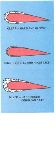
There are three types of structural icing clear, rime and mixed. They are shown in figure 1 and discussed in detail below.
2.4.1 Clear Ice
When an aircraft initially comes in contact with the liquid, there are some water droplets which stick at the point of contact. The remaining droplets flow over the surface of the aircraft which steadily freeze forming a smooth sheet of solid ice on the surface of the aircraft. This solid is the clear ice. However, this type of ice only occurs when the droplets of water, in rain or the cumuliform clouds, are large enough. The properties of clear ice include being hard, heavy and firm making it extremely difficult to remove, even with use of de-icing equipment. Hence, it can be seen why this type of ice would have a deep impact on aircraft aerodynamics are its properties significantly increase the overall weight of the aircraft which has a direct effect the lift and drag of the aircraft. Clear Ice also changes the shape of the aerofoil, again effecting the lift and drag characteristics of an aircraft. Typically, clear ice occurs between temperatures of 0 and -10 degree Celsius (Chapter 10 – ICING, 2017).
2.4.2 Rime Ice
Unlike clear ice, rime ice is formed when the water droplets are small. The remaining droplets, after the initial contact of the aircraft with liquid, freeze swiftly preventing the drops to spread. Rime ice has milky look to it as air is trapped between these frozen droplets. Compared to clear ice, rime ice is significantly lighter in weight, hardly having any effect on the weight of the aircraft. However, the rime ice makes the surface of the aerofoil rough and forms and irregular shape on the surface, which decreases the aerodynamic efficiency of the aerofoil. Hence, increasing drag and reducing lift. The properties of rime ice are that its brittle, making it easier to remove when compared to clear ice. Typically, rime ice occurs between temperatures of -15 and -20 degrees Celsius (Chapter 10 – ICING, 2017).
2.4.3 Mixed Ice
Mixed ice is a mixture of clear and rime ice, as suggested by the name. Mixed ice forms when different sized water droplets rapidly freeze when they come in contact with the surface of the aircraft. In comparison to rime and clear ice, mixed ice has the worse characteristics purely because of the increased roughness on the surface of the aircraft. Typically, mixed ice occurs between the temperatures of -10 and -15 degrees Celsius (Chapter 10 – ICING, 2017).
2.5 Similar Wind Tunnel Experiments
Broeren et al., 2011, undertook a study on different ice accretion on the leading of a wing. They performed a test in NASA’s Icing Research Tunnel (IRT) which is a is a “closed-return, refrigerated wind tunnel that contains a system of spray nozzles that are used to simulate in-flight icing cloud conditions”. The aerofoil used in their experiment was the NACA 23012. The test was performed for two different models, a sub-scaled wing model and a full-scaled wing model. The types of ice accretion they used was different to the ones in this study. However, the effects would be similar and can be compared with the results of this study. They used Horn ice simulation and Spanwise-Ridge ice simulation which is very similar to rime ice. They obtained data for pressure distribution across the aerofoil by adding pressure taps at various locations on the model. These taps record the pressure at that point for given flow and thus, a pressure distribution can be plotted. A similar pressure distribution is shown Chapter 5.2.
To summarise, their results can be used as benchmark to compare effects as their results are highly reliable. This is due to the fact that they used actual ice for simulation and in an iced wind tunnel which replicate real flight conditions.
2.6 Similar Numerical Simulation
A similar numerical simulation to the one performed in this project was undertake by Da-lin and Wei-jian, 2005. Their simulation emphasized on rime ice accretion process on an aerofoil. They incorporated a two-phase model of super-cooled droplets. This is a very useful model as this simulation provides an actual representation of rime ice accretion on the wing. Da-lin and Wei-jian, 2005, explain that “Incorporating the two-phase model of air-supercooled droplets in the Eulerian coordinate system, this technique is applied to simulate the process of the rime ice accretion (the droplets freeze at the instant impinging on the airfoil) on the NACA 0012 airfoil, and the ice profile after ice accretion is achieved successfully”. The reason these water droplets freeze at contact with the aerofoil is due to the temperature. A constant freezing temperature is maintained to allow these super-cooled droplets to freeze. The effects of ice are evaluated by plotting surface pressure distribution for clean and iced aerofoil. Similar, plot is generated for numerical results in this study shown and discussed in Chapter 6.2.1.
3 THEORECTICAL RESULTS
In this chapter, I will calculate the theoretical results of the NACA 0012, used at the wing tip of the Cessna 152 aircraft. The aim of his project is to investigate the aerodynamic performance and therefore it is essential to analyse the changes in the lift and drag forces of the aircraft. Therefore, I will be calculating the coefficient of lift and drag for the NACA 0012 aerofoil. However, it is quite challenging to calculate the lift coefficient theoretically as it is normally obtained using wind tunnel tests. But, it is possible to obtain 2D lift coefficient of the airfoil shape and then convert it to 3D, based on the span and chord of the wing. This can then be used as theoretical data to compare it with the experimental, wind tunnel, test. The drag can be calculated theoretically. I will be investigating the aerodynamic performance at three different Reynold’s Numbers 20000, 250000 and 30000. These correspond to velocities of 11.8 ms-1, 14.8 ms-1 and 17.8 ms-1 respectively. These values are obtained using calculations shown below. The Reynolds number is given by:
Re= ρ*v*lμ
Where,
- ρis the density of the air at sea level. This value is obtained from the International Standard Atmosphere (ISA).
- v is the velocity of the travelling air.
- lis the chord length of the wing.
- μis the dynamic viscosity at given condition (Sea Level for this project). This value is obtained to be 1.81E-5 from ISA
Rearranging Equation 3‑1 in terms of velocity would allow me to calculate the velocity.
v= Re*μρ*l= 200000*1.81×10-51.225*0.25= 11.8 ms-1
Equation 3‑2 shows a sample calculation of velocity of 200000 Reynolds number. The same equation was used to obtain velocity for different Reynolds numbers.
I will be using the XFOIL v6.99, a Subsonic Airfoil Development Software, to obtain 2D lift coefficient and then convert it to 3D. XFOIL is obtained from Drela, 2017. The XFOIL Pressure distribution and command window of Reynold’s Number of 300000 is shown in APPENDIX A – XFOIL Pressure Distribution and Command Window for Reynold’s Number of 300000..
3.1 Reynolds Number of 200000
This section shows the lift and drag coefficients obtained from XFOIL v6.99. As mentioned earlier, these are two dimensional coefficients and therefore these will have to be converted to three dimensional to allows us to compare it with our experimental and numerical (CFD) results. The lift and drag coefficients will be obtained for three different Reynold’s Numbers. This would allow us to analyse the effects of ice on aerodynamic performance at different speeds. Hence, three different Reynolds Numbers were chosen.
3.1.1 Theoretical Lift Coefficient
| Angle of Attack (degrees) | Cl 2D |
| -4 | -0.5358 |
| -2 | -0.3084 |
| 0 | 0 |
| 2 | 0.3084 |
| 4 | 0.5357 |
| 6 | 0.6975 |
| 8 | 0.8494 |
| 10 | 1.0068 |
| 12 | 1.0993 |
| 14 | 0.9632 |
| 16 | 0.7085 |
Table 1 shows 2D coefficients obtained from XFOIL. These can now be converted into 3D. To do this, the two-dimensional lift-curve slope must be calculated. This is essentially the gradient of plot, lift coefficient against the angle of attack.
Table 1 2D Lift Coefficient for 200000 Reynold’s Number
The equations and calculations needed to obtain the theoretical lift coefficients are shown below. Equation 3‑3 shows the calculated lift curve slope for the data obtained from XFOIL shown in Table 1.
2D Lift Curve Slope= ΔY∆X= ΔClΔα = 0.9632–0.535814–4* 180°π= 4.77 radians-1
This 2D lift curve slope can now be used to calculate the 3D lift curve slope by taking 3D effects into account. These effects include the Aspect Ratio (AR) and the Oswald Efficiency (e) of the wing. For an aspect ratio of less than 4, It can be calculated using Equation 3‑4 (Mh-aerotools.de, 2017).
3D Lift Curve Slope= 2D lift curve1+2D lift curveπ*AR*e2+2D lift curveπ*AR*e
Where,
- AR is the Aspect Ratio of the Wing
- e is the Oswald Efficiency of the wing.
The aspect ratio is the ratio between the wing span (b) and the wing area (S). The model of the wing that I have manufactured, for this project, is scaled down by a factor of 18 from the actual wing span of Cessna 152. The wingspan of Cessna 152 is 33.4 inches which is approximately 10.2 metres and therefore my model is 0.575 m. The chord length of my wing is 0.25 m and therefore my wing planform area is 0.25*0.575 = 0.14375 m2. These values were chosen to meet the requirements of the wind tunnel that was used to obtain experimental results for this project, this is discussed in further detail in chapter 5. The aspect ratio can be calculated using Equation 3‑5 shown below.
AR= b2S= 0.57520.14375=2.3
Oswald efficiency factor is calculated using equation 3-4 (Sadraey, 2009).
e =1.781-0.0045AR0.68-0.64 =1.781-0.00452.40.68-0.64 =1.13
Hence, substituting the values from Equation 3‑5 and Equation 3‑6 into Equation 3‑4, the 3D lift curve slope can be calculated.
3D Lift Curve Slope= 4.771+4.77π*2.3*1.132+4.77π*2.3*1.13=2.74 radian-1
This lift curve slope can be used to calculate the theoretical lift coefficient which can be used to for comparison. The 3D lift coefficient is given by substituting values from Table 1, Equation 3‑3 and Equation 3‑5 into Equation 3‑7 (Mh-aerotools.de, 2017).
CL= Cl3D lift curve2D lift Curve
Where,
Clis the 2D lift coefficient obtained from XFOIL. A sample calculation for
α= -4°is shown below. The 2D lift coefficient (Cl) for
α= -4°is -0.5358, hence 3D lift coefficient (CL) is
CL= Cl3D lift curve2D lift Curve= -0.53582.744.77= -0.307
| Angle of Attack (Deg) | Cl 2D | Lift Curve 2D | Lift Curve 3D | CL 3D |
| -4 | -0.5358 | 4.77 | 2.74 | -0.3075 |
| -2 | -0.3084 | 4.77 | 2.74 | -0.1770 |
| 0 | 0.0000 | 4.77 | 2.74 | 0.0000 |
| 2 | 0.3084 | 4.77 | 2.74 | 0.1770 |
| 4 | 0.5357 | 4.77 | 2.74 | 0.3074 |
| 6 | 0.6975 | 4.77 | 2.74 | 0.4003 |
| 8 | 0.8494 | 4.77 | 2.74 | 0.4874 |
| 10 | 1.0068 | 4.77 | 2.74 | 0.5778 |
| 12 | 1.0993 | 4.77 | 2.74 | 0.6308 |
| 14 | 0.9632 | 4.77 | 2.74 | 0.5527 |
| 16 | 0.7085 | 4.77 | 2.74 | 0.4066 |
Table 2shows all the calculated values for different angles of attack. This will data will be used as theoretical data for Reynolds number 20000 during analysis.
The above calculation can be performed for all angles of attack to obtain the theoretical lift coefficient.
3.1.2 Theoretical Drag Coefficient
The theoretical drag calculations are different to that of lift. Since I am only evaluating the aerodynamics of the wing of Cessna 152, I will only be calculating the drag of the wing. There are two different types of drag that combine to give the total drag of a given aircraft’s component. The two types of drag are parasitic drag and induced drag.
The parasitic drag is the zero lift drag of an aircraft. The parasitic drag is due to the skin friction of the aerofoil; thus, it is sometimes referred to as skin friction drag. All the different components of the aircraft such as wing, fuselage and tail contribute to the total parasitic drag. The parasitic drag varies at different flight conditions like cruise or landing. This is due to the fact and the parasitic drag is the function of MACH and Reynolds number and they both change at different conditions as the density and the speed vary. Hence, it is important to calculate the parasitic drag for all the three different Reynolds number that I have chosen.
Induced drag is the drag due to the lift produced by the wing. “The drag that results from the generation of a trailing vortex system downstream of a lifting surface with a finite aspect ratio. In another word, this type of drag is induced by the lift force” (Sadraey, 2009). Induced drag is a function of the wings aspect ratio and Oswald efficiency.
The total drag coefficient (
CD) of the wing is given by
CD= CDoW+ CDi
Where,
- CDoWis the parasitic drag of the wing.
- CDiis the induced drag of the wing.
| Angle of Attack (Deg) | CDoW |
| -4 | 0.01176 |
| -2 | 0.01066 |
| 0 | 0.0102 |
| 2 | 0.01066 |
| 4 | 0.01176 |
| 6 | 0.01513 |
| 8 | 0.02076 |
| 10 | 0.02975 |
| 12 | 0.04416 |
| 14 | 0.11774 |
| 16 | 0.18817 |
The parasitic drag is obtained from XFOIL, similar to that of lift coefficient. Below is the table showing the values of parasitic drag obtained for different angles of attack.
Table 3 summaries the obtained drag values from XFOIL. These values correspond to Reynolds number of 200000. These contribute to the overall drag of the wing.
Table 3 Skin Friction Drag from XFOIL
The induced drag is given by
CDi= CL2π*AR*e
Where,
- CLis the 3D coefficient of lift shown in Table 2.
- ARis the aspect ratio calculated in Equation 3‑5.
- eis the Oswald efficiency calculated in Equation 3‑6.
A calculation of induced and total drag for
α= -4°is shown below
CDi= CL2π*AR*e= -0.30752π*2.3*1.13=0.0116
The induced drag also changes with lift and therefore it is calculated for all the angles of attack as the lift changes with angles of attack. It is calculated using the same method shown in the above equation using values for lift coefficient from Table 2 for different angles of attack.
Hence, substituting the values from Table 3 and Equation 3‑9 into Equation 3‑8 gives the value of the theoretical drag for
α= -4°.
CD= CDoW+ CDi=0.01176+0.0116=0.0233
The above calculation is repeated for different angles of attack and the theoretical value of drag is obtained. Table below shows all the calculated values of drag.
| Angle of Attack (Deg) | CDoW | CDi | CD |
| -4 | 0.01176 | 0.0116 | 0.0233 |
| -2 | 0.01066 | 0.0038 | 0.0145 |
| 0 | 0.0102 | 0.0000 | 0.0102 |
| 2 | 0.01066 | 0.0038 | 0.0145 |
| 4 | 0.01176 | 0.0116 | 0.0233 |
| 6 | 0.01513 | 0.0196 | 0.0348 |
| 8 | 0.02076 | 0.0291 | 0.0499 |
| 10 | 0.02975 | 0.0409 | 0.0706 |
| 12 | 0.04416 | 0.0487 | 0.0929 |
| 14 | 0.11774 | 0.0374 | 0.1552 |
| 16 | 0.18817 | 0.0202 | 0.2084 |
Table 4 Theoretical Drag Coefficient for Reynolds Number of 200000
Table 4 shows the theoretical drag coefficients that will be used for analysis.
3.2 Reynolds Number of 250000
The theoretical for Reynold’s number of 250000 are calculated in the same way as shown in section 3.1 of this chapter. Equations from section 3.1.1 and 3.1.2 of this chapter were used to calculate the theoretical lift and drag coefficients for this Reynolds number. The only difference here would be that the speed changes due to Reynolds number. Below is the summary table showing both the lift and drag coefficients.
| Angle of Attack (Deg) | Cl 2D | 2D Lift Curve | 3D lift Curve | CL 3D | CDoW | CDi | CD |
| -4 | -0.5371 | 5.12 | 2.83 | -0.2972 | 0.01105 | 0.0108 | 0.0219 |
| -2 | -0.2664 | 5.12 | 2.83 | -0.1474 | 0.00959 | 0.0027 | 0.0123 |
| 0 | 0.0000 | 5.12 | 2.83 | 0.0000 | 0.00863 | 0.0000 | 0.0086 |
| 2 | 0.2664 | 5.12 | 2.83 | 0.1474 | 0.00959 | 0.0027 | 0.0123 |
| 4 | 0.5370 | 5.12 | 2.83 | 0.2972 | 0.01105 | 0.0108 | 0.0219 |
| 6 | 0.7029 | 5.12 | 2.83 | 0.3890 | 0.01412 | 0.0185 | 0.0326 |
| 8 | 0.8563 | 5.12 | 2.83 | 0.4738 | 0.01899 | 0.0275 | 0.0465 |
| 10 | 1.0104 | 5.12 | 2.83 | 0.5591 | 0.02663 | 0.0383 | 0.0649 |
| 12 | 1.1260 | 5.12 | 2.83 | 0.6231 | 0.0378 | 0.0475 | 0.0853 |
| 14 | 1.0709 | 5.12 | 2.83 | 0.5926 | 0.062 | 0.0430 | 0.1050 |
| 16 | 0.7128 | 5.12 | 2.83 | 0.3944 | 0.18616 | 0.0191 | 0.2052 |
Table 5 Theoretical Lift and Drag Coefficients for Re 250000
3.3 Reynolds Number of 300000
The theoretical calculations for this Reynolds are, again, calculated using methods and equations shown in section 3.1.1 and 3.1.2 of this chapter. Hence, they have not been repeated here and a summary table is shown below.
| Angle of Attack (Deg) | Cl 2D | 2D Lift Curve | 3D lift Curve | CL 3D | CDoW | CDi | CD |
| -4 | -0.540 | 5.137 | 2.837 | -0.298 | 0.01056 | 0.0109 | 0.0214 |
| -2 | -0.238 | 5.137 | 2.837 | -0.131 | 0.00875 | 0.0021 | 0.0109 |
| 0 | 0.000 | 5.137 | 2.837 | 0.000 | 0.00768 | 0.0000 | 0.0077 |
| 2 | 0.238 | 5.137 | 2.837 | 0.132 | 0.00875 | 0.0021 | 0.0109 |
| 4 | 0.540 | 5.137 | 2.837 | 0.298 | 0.01056 | 0.0109 | 0.0214 |
| 6 | 0.708 | 5.137 | 2.837 | 0.391 | 0.01337 | 0.0187 | 0.0321 |
| 8 | 0.863 | 5.137 | 2.837 | 0.477 | 0.01785 | 0.0278 | 0.0457 |
| 10 | 1.013 | 5.137 | 2.837 | 0.559 | 0.02398 | 0.0383 | 0.0623 |
| 12 | 1.125 | 5.137 | 2.837 | 0.621 | 0.03402 | 0.0473 | 0.0813 |
| 14 | 1.074 | 5.137 | 2.837 | 0.593 | 0.05881 | 0.0431 | 0.1019 |
| 16 | 0.702 | 5.137 | 2.837 | 0.388 | 0.18518 | 0.0184 | 0.2036 |
4 EXPERIMENTAL RESULTS
This chapter explains the process of obtaining my experimental results. The aircraft I have chosen is Cessna 152 and so I will be using its aerofoil to produce my model of the wing. As mentioned before, I will be assuming a constant aerofoil shape, NACA 0012, across the span wing to reduce the complexity of the project. Figure 2 shows the aerofoil shape of NACA 0012.
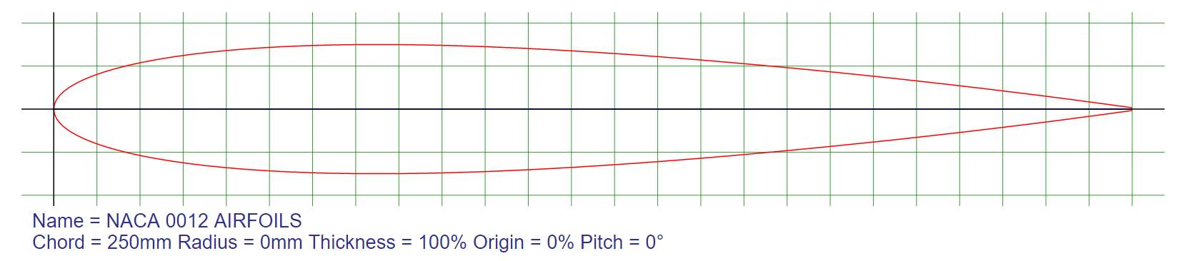
Figure 2 NACA 0012 Aerofoil (“NACA 0012 AIRFOILS (N0012-Il)”)
To obtain the experimental results, I will be performing the wind tunnel test with different configurations. These configurations are clean wing, rime iced wing, clear iced wing and mixed ice wing (Section 2.3). This is undertaken to effectively analyse the effects of different types of ice on aerodynamic performance of an aircraft. Hence, I will be casting these different types of ice on my wing to evaluate their effects. However, it is very difficult to apply actual ice to the wing due to its properties. Therefore, I will be an alternate material that can replicate ice and its effects. The choice of material is discussed in section 4.1.3 of this chapter.
4.1 Wing Model
Initially, I had decided that I would develop the wing model for my wind tunnel test using a 3D printer which uses plastic as a material. However, I will now be using wood as my primary material for my model and physically manufacture the model and not use a 3D printer. I made this decision after comparing different approaches and taking advices from different technicians at the university and it was concluded that for the purpose of this project, physically manufacturing would be appropriate especially with the wind tunnel requirements (discussed in section 4.2). It is also a lot cheaper to take this approach than to use a 3D printer as 3D printing is very expensive. The process of manufacturing my wing is discussed in this section.
4.1.1 CAD Model
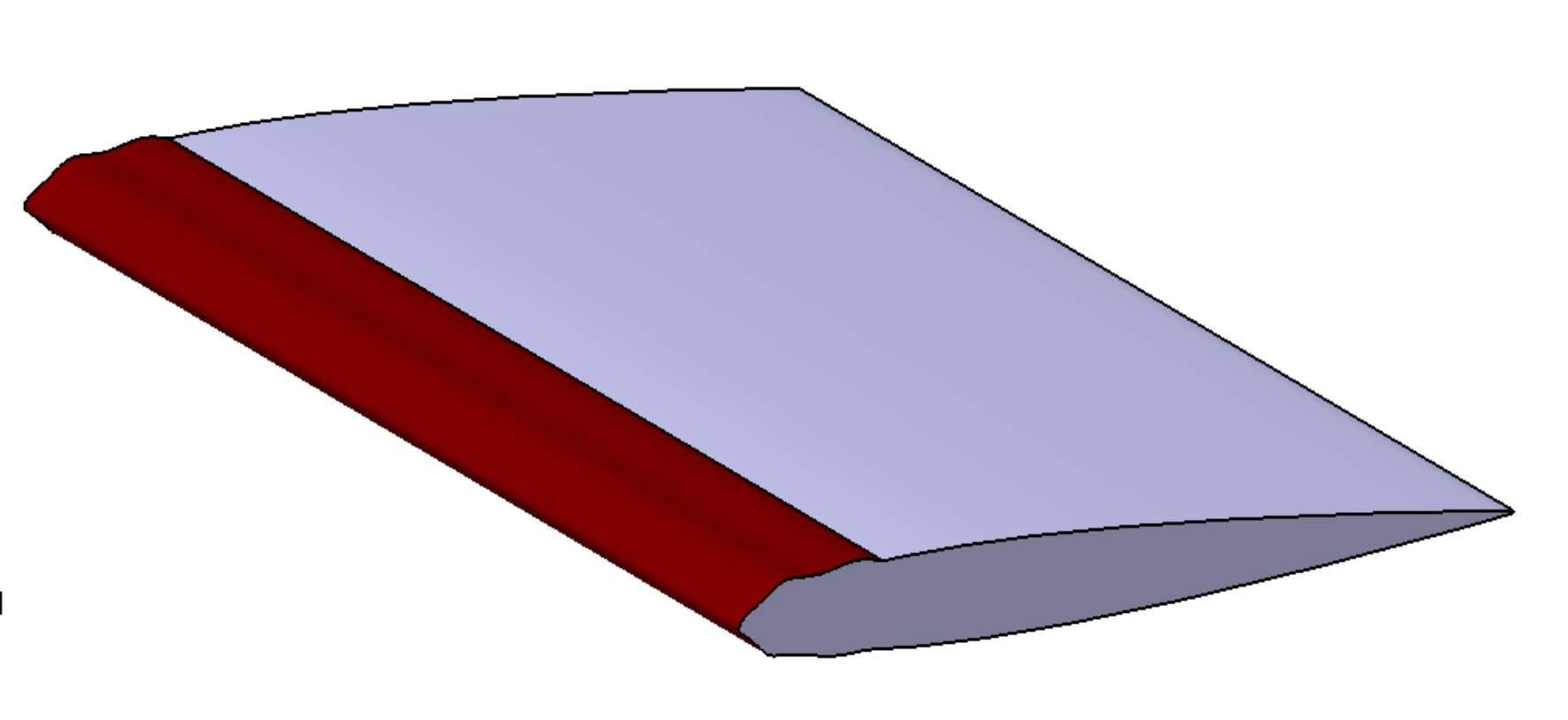
Firstly, a 3D model of the wing was developed using CATIA V5, a powerful 3D modelling software widely used in industry. The wing was modelled by importing the coordinates of the aerofoil to produce a precise shape of the aerofoil (The coordinates of the aerofoil are shown in APPENDIX B – NACA 0012 Aerofoil Coordinates. Figure 3 shows the 3D model of my wing.
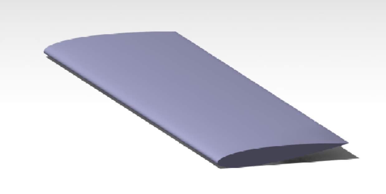
Figure 3 CATIA Model of the Wing
4.1.2 Manufacturing Process
The wing was manufactured using Balsa wood, this was done by consulting technicians at the university and their approval. The first step of developing the wing was creating the inner ribs of the wings. The ribs created using a Laser Cutting machine available at the University of Hertfordshire. This was done by importing a drawing of the rib, obtained from CATIA V5 using the NACA 0012 coordinates.
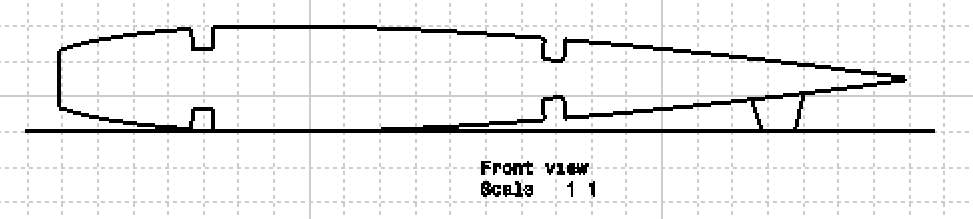
Figure 4 shows the CATIA drawing of the rib which was imported in the laser cutting machine to cut the wood in the shape of the rib. The four boxed pockets in the above figure represent the space where the spars would be connected. A total number of 10 spars were chosen across the span of the wing and the Balsa wood used for the ribs had a thickness of 10mm. The horizontal distance between the two spars was chosen two be 100mm and the distance between the trailing edge of aerofoil and the trailing edge spar was also 100mm. These distances were chosen because the wood skin that will be used to cover the ribs and spars and obtain the shape of the wing has width of 100 mm. Hence, it was important to place the spars as they were to allow for the skin to glue in place since super glue was used for the assembly of the model. The spars were 5mm square rod.
Once the ribs were laser cut, the wing was assembled. The assembly process involved attaching the ribs with the spars using super glue and then placing the skin to complete the wing. The final process was to sand the entire wing thoroughly using sand paper to avoid any roughness on the surface and ensure it is smooth. This is very important as the data obtain as a result of a rough surface is not very accurate. Hence, a smooth surface would ensure that there is no interference in the flow during the wind tunnel test.
4.2 Material Selection
The selection of material to replace ice on a wing is a challenging task as no material would be provide properties same as that of ice. However, reasonable selection of materials would give us accurate results to fulfil the purpose of this project. Therefore, few different properties of materials were compared with ice and a choice of material was made. The list of materials used for comparison with ice was selected by doing some background research on similar experiments and consulting lecturers and technicians at the university.
| Material | Properties |
| Ice |
Source: (Eniscuola, 2017) |
| Modelling Wax |
Source: (Kemdent.co.uk, 2016) |
| Polystyrene Foam |
Source: (Hotwire Systems OÜ, 2017) |
Table 7 Properties of Different Modelling Materials
After comparing the above table, I concluded that I will be using the modelling wax to replicate ice accretion on a wing. This is purely due to the fine modelling characteristics of wax. The polystyrene foam is similar in weight when compared with ice. However, wax provides detail in modelling and the roughness that ice has. Modelling wax is also cost efficient and therefore I decided with approval of technicians that wax will be used to replicate ice accretions.
4.3 Wind Tunnel Test
“A wind tunnel is a specially designed and protected space into which air is drawn, or blown, by mechanical means in order to achieve a specified speed and predetermined flow pattern at a given instant. The flow so achieved can be observed from outside the wind tunnel through transparent windows that enclose the test section and flow characteristics are measurable using specialized instruments. An object, such as a model, or some full-scale engineering structure, typically a vehicle, or part of it, can be immersed into the established flow, thereby disturbing it. The objectives of the immersion include being able to simulate, visualize, observe, and/or measure how the flow around the immersed object affects the immersed object.” (Lerner and Boldes, 2011).
There are different classifications for wind tunnel. They are listed below:
- Open or Closed Wind Tunnels
- Speed Limits – Supersonic or Subsonic
- Educational or Research
- Nature of Flow
There are two types of wind tunnel that I investigated, Closed Return Interchangeable Modular (CRIM) and Open Jet wind tunnel. I compared these two as they are available to use at the university.
CRIM Wind Tunnel is a subsonic wind tunnel which has the ability to produce of speeds up to 20m/s and angles of attack of -4 to 16 degrees maximum. Can measure Reynolds number up to 0.34E5 per metre and Dynamic Pressure: up to 390 N/m2. Figure 6 shows the structure
;kfkfkf;lkf;lkf;lkf;lkf;kf and main components of the closed return wind tunnel.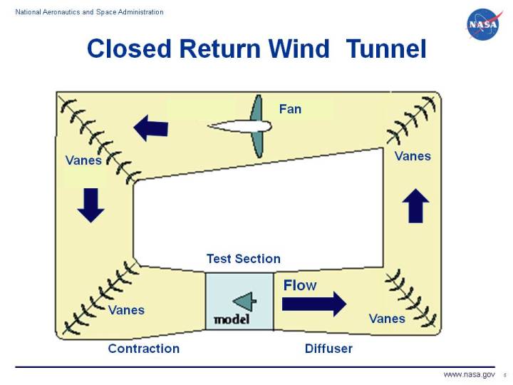
The characteristic of each component within the CRIM wind tunnel are:
- The inlet contains honeycomb flow straighteners and wire mesh smoothing screens to condition the airflow.
- The contraction cone takes a large volume of low velocity air and reduces it to a small volume of high velocity air without creating turbulence.
- The test item and sensors are placed in the test section.
- The diffuser slows down the air exiting the test section prior to exhaust or recirculation.
- Vanes are used to turn the airflow around the corners of the tunnel to minimise turbulence.
- Fast-moving air coming out of the tunnel can be recirculated into its intake to help boost the total airspeed. This also helps to reduce the drive power required.
If the air is drawn directly from the surroundings into the wind tunnel and rejected back into the surroundings, the wind tunnel is said to have an open-air circuit. Thus, it is known as Open Jet wind tunnel (Lerner and Boldes, 2011).
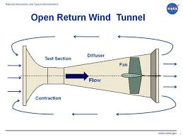
Figure 7 Open Return Wind Tunnel
The properties of open return wind tunnel are:
- Mach Number: 0.16 (max)
- Maximum Flow Speed: up to 55 m/s
- Reynolds No: up to 3.88×10⁶ /m
- Total Pressure: ~1 bar
- Dynamic Pressure: up to 1.9 kNm-2
To Summarise, a wind tunnel has many applications and is widely used in the industry and universities to obtain experimental data. The main reason being that the data acquired from wind tunnel test is considered highly reliable and acceptable. Thus, it is a good source to obtain experimental results.
After comparing the two wind tunnels, I concluded to use the CRIM wind tunnel to undertake my test and obtain experimental results. The reason being that the CRIM Wind Tunnel has appropriate data acquisition capabilities which are required in my project, it provides acceptable values of lift and drag force which are the main values of comparison in my analysis. My project requires me to obtain aerodynamic data of the wing and the CRIM wind tunnel adequately provides that. Hence, I would be using the CRIM wind tunnel.
The span size of the two arm inside the wind tunnel was measured with the technician. The distance between the two arms, where each end of the span of my model is attached, was measured to be 600mm. As a result, A span of 575mm was decided with the approval of the technician for my wing model. The span was chosen to be slightly smaller than that measured in the wind tunnel, purely because it would allow enough room for attachments between the two and ensure smooth flow and movement of the model caused by different angles of attack. The chord of wing was decided to be 250mm and was kept constant.
The wind tunnel test was performed for different types of iced wing configurations and each test was repeated three times to ensure that the data obtained is reliable. The results obtained from wind tunnel tests are discussed below in their respective sections.
4.3.1 Bare Wing
The first test that was done was with the clean wing. This is very important test to perform as this is used as benchmark test. This is due to the fact that this test would show if the experimental results are acceptable or not when compared to theoretical. So, if these results are not acceptable then the iced wing data is not considered reliable. This test also provides consistency when comparing experimental data for iced aerofoil as they would all be performed in the same environment. Hence, it is vital to perform this test first. The wind tunnel outputs the value of lift and drag force. The lift coefficients for each of these force is calculated (discussed further down in this section).
| Angle of Attack | Lift (N) | Drag (N) | Average CL | Average CD | ||||||
| Test 1 | Test 2 | Test 3 | Average | Test 1 | Test 2 | Test 3 | Average | |||
| -4 | -2.5190 | -2.6500 | -2.5680 | -2.5790 | 0.4896 | 0.5107 | 0.4884 | 0.4962 | -0.2104 | 0.0399 |
| -2 | -1.0790 | -1.1450 | -1.0740 | -1.0993 | 0.4467 | 0.4470 | 0.4390 | 0.4442 | -0.0897 | 0.0364 |
| 0 | 0.2268 | 0.1450 | 0.1108 | 0.1609 | 0.4323 | 0.4349 | 0.4540 | 0.4404 | 0.0131 | 0.0353 |
| 2 | 1.6330 | 1.5310 | 1.4740 | 1.5460 | 0.4828 | 0.4972 | 0.4978 | 0.4926 | 0.1261 | 0.0394 |
| 4 | 3.2320 | 3.3030 | 3.2590 | 3.2647 | 0.6003 | 0.6056 | 0.6038 | 0.6032 | 0.2663 | 0.0490 |
| 6 | 4.7430 | 4.8470 | 4.6830 | 4.7577 | 0.7600 | 0.7650 | 0.7556 | 0.7602 | 0.3881 | 0.0620 |
| 8 | 6.2020 | 6.2120 | 6.1270 | 6.1803 | 0.9421 | 0.9315 | 0.9498 | 0.9411 | 0.5041 | 0.0768 |
| 10 | 7.4270 | 7.5660 | 7.4110 | 7.4680 | 1.1590 | 1.1740 | 1.1620 | 1.1650 | 0.6092 | 0.0945 |
| 12 | 8.6040 | 8.8180 | 8.6740 | 8.6987 | 1.4030 | 1.4790 | 1.4450 | 1.4423 | 0.7095 | 0.1144 |
| 14 | 9.0630 | 9.0760 | 8.9130 | 9.0173 | 2.5060 | 2.5140 | 2.4410 | 2.4870 | 0.7355 | 0.2044 |
| 16 | 8.7700 | 8.5880 | 8.5050 | 8.6210 | 3.2250 | 3.2090 | 3.1760 | 3.2033 | 0.7032 | 0.2631 |
Table 7 shows a sample table for measured values from the wind tunnel. As shown, the test was repeated three times and an average was taken to make the tests more reliable. The shown coefficient of lift and drag were calculated using the average lift and drag. A sample calculation is shown below.
The lift of a wing is given by
L= 12*ρ*v2*S*CL
where,
- ρrepresents the density of the air at given altitude (Sea Level in this project). The value is same as shown in chapter 3.1.
- vrepresents the velocity of the flow, 11.8 ms-1 corresponding to RE 200000
- CLrepresents the lift coefficient at a given condition.
- Srepresents the wing planform area.
Rearranging Equation 4‑1 in terms of
CLgives:
CL= 2Lρ*v2*S ⟹ CD= 2Dρ*v2*S
A calculation for
α= -4°is shown by substituting average lift and drag values into Equation 4‑2
CL= 2Lρ*v2*S= 2* -2.57901.225*11.82*0.14375= -0.2104
Similarly, drag coefficient is given by
CD= 2Dρ*v2*S= 2* 0.49621.225*11.82*0.14375= 0.0399
| Angle of Attack (Deg) | Re 200000 | Re 250000 | Re 300000 | |||
| CL | CD | CL | CD | CL | CD | |
| -4 | -0.2104 | 0.0399 | -0.2580 | 0.0415 | -0.3066 | 0.0437 |
| -2 | -0.0897 | 0.0364 | -0.1431 | 0.0366 | -0.1896 | 0.0371 |
| 0 | 0.0131 | 0.0353 | -0.0316 | 0.0341 | -0.0827 | 0.0343 |
| 2 | 0.1261 | 0.0394 | 0.0719 | 0.0370 | 0.0288 | 0.0345 |
| 4 | 0.2663 | 0.0490 | 0.1880 | 0.0426 | 0.1349 | 0.0385 |
| 6 | 0.3881 | 0.0620 | 0.3227 | 0.0549 | 0.2598 | 0.0477 |
| 8 | 0.5041 | 0.0768 | 0.4515 | 0.0694 | 0.3936 | 0.0609 |
| 10 | 0.6092 | 0.0945 | 0.5628 | 0.0855 | 0.5155 | 0.0759 |
| 12 | 0.7095 | 0.1144 | 0.6658 | 0.1055 | 0.6242 | 0.0947 |
| 14 | 0.7355 | 0.2044 | 0.7671 | 0.1327 | 0.7296 | 0.1176 |
| 16 | 0.7032 | 0.2631 | 0.7211 | 0.2307 | 0.7417 | 0.1966 |
The above calculations are repeated for all different angles of attack to obtain values for lift and drag coefficient shown in Table 7. These calculations are repeated for all the different Reynolds numbers and therefore they are not shown again. Table 8 shows all the calculated values of lift and drag coefficient with detailed table shown in APPENDIX C.
4.3.2 Rime Iced Wing
The rime ice results were obtained by modelling wax similar to rime ice on the leading edge of the wing. Section 2.3.2 discusses the properties of rime ice. The ice was modelled based on these properties to model ice very similar to rime ice. The surface was made rough and irregular as it normally occurs in real situations. The layer of rime is very thin so for my model a range of thickness between 1mm to 1.5 mm was measured at various points across the wingspan. The results obtained are similar to that shown in section 4.2.1 and the same method and calculations were undertaken to obtain values for lift and drag coefficients. Therefore, the final obtained values for all different Reynolds numbers and angles of attack are shown below with detailed results obtained shown in APPENDIX D.
| Angle of Attack (Deg) | Re 200000 | Re 250000 | Re 300000 | |||
| CL | CD | CL | CD | CL | CD | |
| -4 | -0.0931 | 0.0398 | -0.1323 | 0.0387 | -0.2214 | 0.0414 |
| -2 | -0.0503 | 0.0374 | -0.1289 | 0.0358 | -0.1403 | 0.0370 |
| 0 | -0.0039 | 0.0380 | -0.0335 | 0.0363 | -0.0465 | 0.0361 |
| 2 | 0.0807 | 0.0406 | 0.0319 | 0.0396 | 0.0675 | 0.0378 |
| 4 | 0.1754 | 0.0475 | 0.1250 | 0.0459 | 0.1810 | 0.0429 |
| 6 | 0.2504 | 0.0581 | 0.2333 | 0.0552 | 0.2979 | 0.0510 |
| 8 | 0.3229 | 0.0709 | 0.3340 | 0.0693 | 0.4221 | 0.0629 |
| 10 | 0.4244 | 0.0897 | 0.4376 | 0.0860 | 0.5420 | 0.0787 |
| 12 | 0.5249 | 0.1121 | 0.5429 | 0.1079 | 0.6588 | 0.0981 |
| 14 | 0.5996 | 0.1488 | 0.6416 | 0.1372 | 0.7772 | 0.1225 |
| 16 | 0.6199 | 0.2202 | 0.6528 | 0.2090 | 0.8322 | 0.1754 |
Table 10 Experimental Results for Rime Ice
4.3.3 Clear Iced Wing
Clear ice was modelled by adding more layers of wax on that of rime ice. The properties of clear ice are discussed in Chapter 2.3.1. These properties were modelled and applied on the leading edge of the wing, as close to the real ice as possible, to obtain acceptable results for clear ice. Clear ice is thicker in layer compared to rime ice and it was measured in the range of 1.5mm to 2.5mm. The shape was made irregular and surface a bit smother compared to rime ice but still rough. The final calculated values are shown below with detailed values shown in APPENDIX E.
| Angle of Attack (Deg) | Re 200000 | Re 250000 | Re 300000 | |||
| CL | CD | CL | CD | CL | CD | |
| -4 | -0.1728 | 0.0444 | -0.1728 | 0.0444 | -0.2332 | 0.0473 |
| -2 | -0.1304 | 0.0418 | -0.1304 | 0.0418 | -0.1794 | 0.0435 |
| 0 | -0.0582 | 0.0433 | -0.0582 | 0.0433 | -0.0862 | 0.0430 |
| 2 | 0.0392 | 0.0459 | 0.0392 | 0.0459 | 0.0279 | 0.0454 |
| 4 | 0.1483 | 0.0536 | 0.1483 | 0.0536 | 0.1400 | 0.0505 |
| 6 | 0.2566 | 0.0618 | 0.2566 | 0.0618 | 0.2605 | 0.0593 |
| 8 | 0.3817 | 0.0746 | 0.3817 | 0.0746 | 0.3815 | 0.0711 |
| 10 | 0.4899 | 0.0912 | 0.4899 | 0.0912 | 0.5088 | 0.0870 |
| 12 | 0.6203 | 0.1111 | 0.6203 | 0.1111 | 0.6331 | 0.1062 |
| 14 | 0.7270 | 0.1344 | 0.7270 | 0.1344 | 0.7512 | 0.1286 |
| 16 | 0.8085 | 0.1667 | 0.8085 | 0.1667 | 0.8336 | 0.1549 |
Table 11 Experimental Results for Clear Ice
4.3.4 Mixed Iced Wing
Mixed ice was modelled in a way similar to clear and rime ice. However, mixed ice is a lot thicker and very rough compared to others, making it very dangerous. Hence, the mixed ice model was made very thick and rough with an irregular shape. The thickness was measured to be in the range between 2.5mm and 5mm across the wing span. The final results are shown below with detailed results shown in APPENDIX F.
| Angle of Attack (Deg) | Re 200000 | Re 250000 | Re 300000 | |||
| CL | CD | CL | CD | CL | CD | |
| -4 | -0.2415 | 0.0700 | -0.2974 | 0.0725 | -0.3517 | 0.0756 |
| -2 | -0.1374 | 0.0645 | -0.1888 | 0.0647 | -0.2407 | 0.0665 |
| 0 | -0.0256 | 0.0627 | -0.0808 | 0.0615 | -0.1282 | 0.0615 |
| 2 | 0.0836 | 0.0641 | 0.0324 | 0.0611 | -0.0180 | 0.0599 |
| 4 | 0.1927 | 0.0699 | 0.1430 | 0.0659 | 0.0942 | 0.0620 |
| 6 | 0.3106 | 0.0792 | 0.2569 | 0.0740 | 0.2089 | 0.0685 |
| 8 | 0.4223 | 0.0944 | 0.3744 | 0.0858 | 0.3247 | 0.0789 |
| 10 | 0.5376 | 0.1153 | 0.4941 | 0.1025 | 0.4444 | 0.0936 |
| 12 | 0.6517 | 0.1402 | 0.6075 | 0.1269 | 0.5579 | 0.1148 |
| 14 | 0.7344 | 0.1821 | 0.7180 | 0.1637 | 0.6703 | 0.1422 |
| 16 | 0.7734 | 0.2400 | 0.7919 | 0.2103 | 0.7669 | 0.1811 |
Table 12 Experimental Results for Mixed Ice
5 NUMERICAL (CFD) RESULTS
Numerical method is essentially a form of computational analysis. Computational Fluid Dynamics (CFD) can be used for numerical analysis as it allows the user to model, solve and simulate experiments in various conditions. CFD is widely used in aerodynamic projects as it allows the user to obtain vital aerodynamic properties like pressure, lift and drag. Hence, it can be considered a reliable method, in terms of numerical analysis, alongside experimental and theoretical. It gives the user that additional outcome to compare and allow for that accurate conclusion of analysis. In this lab, Star CCM+, an industrial and commercial CFD software, will be used to replicate the CRIM wind tunnel environment.
Initially, CFD was not included as a part of this project. However, it was eventually implemented into the study to increase the accuracy of the analysis and conclusion. The whole CFD process took around two months to obtain the results. This involved familiarising with Star CCM+ and setting up the whole model and environment correctly. Hence, only few simulations, for selected angles of attack and conditions, have been performed due to lack of time.
5.1 CFD Setup
A CRIM wind tunnel environment was setup in Star CCM+.
5.1.1 Geometry
Star CCM+ allows the user to input 3D models from other CAD software. Hence, the 3D model prepared to manufacture my experimental wing (Chapter 4.1.1) was imported in Star CCM+ for simulation. A 3D model is inserted as a three-dimensional flow analysis would be performed. This is to compare results with experimental data which was obtained for a three-dimensional finite wing. Figure 7 shows the geometry in Star CCM+.
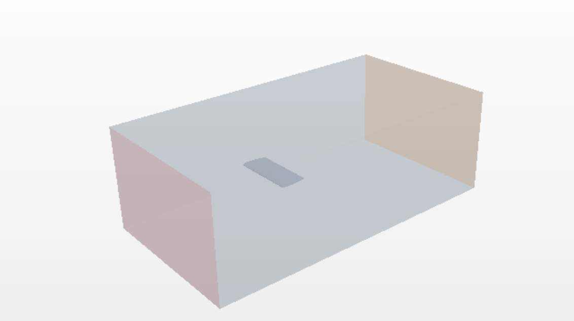
Figure 8 Geometrical Setup in Star CCM+
The annotations of Figure 8 shows the different parts of the geometry setup in Star CCM+. The box outside around the wing is the fluid domain which essentially is the model of the wind tunnel which define the boundary conditions. The left side plane of the fluid domain (Red) is defined as the velocity inlet from where the flow of air is directed towards the wing at a given velocity. The right-side plane of the fluid domain is defined as the pressure outlet from the where the flow exits. The above setup is vital in CFD process and must be defined correctly as it directly affects the flow and the values that are acquired from the simulation.
5.1.2 Mesh
The mesh is another most important parameter in the CFD Process. The mesh is generated within the fluid domain and it consists of finite volume cells on which the CFD equations are approximated. Hence, it is very important to generate an appropriate mesh as it has a major impact on the results obtained.
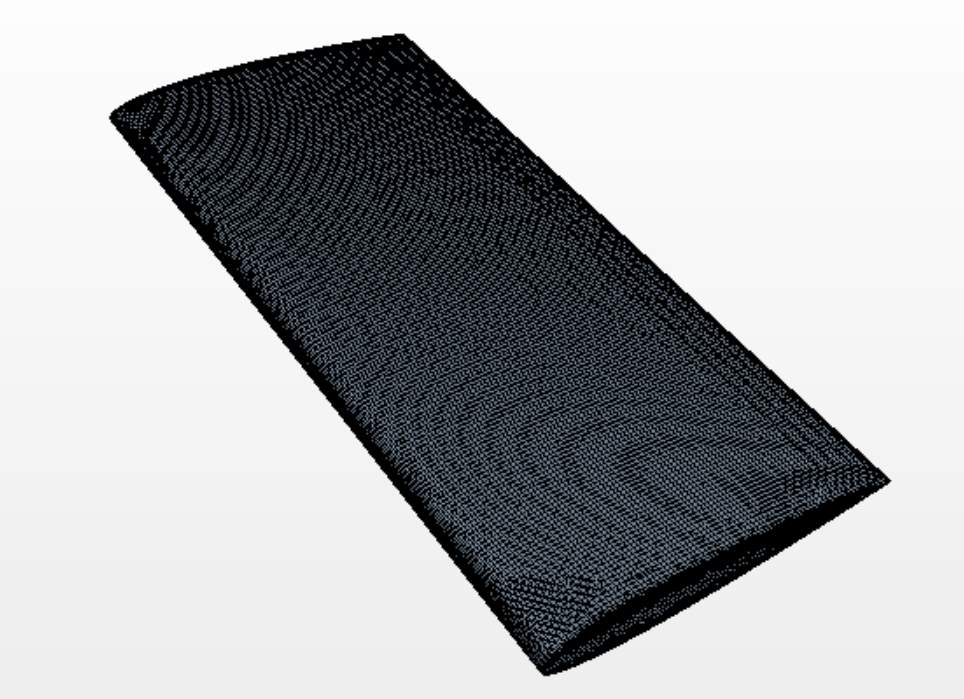
Figure 9 shows the 3D mesh around the wing, the mesh is very fine and the finer the mesh is the more accurate results obtained.
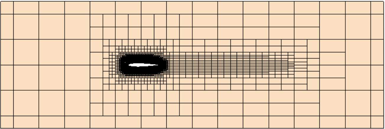
Figure 10 Volume Mesh around the Wing
Figure 10 shows the volume mesh, it is evident that the mesh is made fine around the wing and the wake region after the trailing edge. This increases the accuracy of results obtained. The region near the walls is not made fine and the cell size is significantly larger compared to the wing. This is done to reduce the number of cells and the simulation time.
5.1.3 Physics Models and Boundary Condition
The physics models in CFD describe the flow in the fluid the domain. Physics models include the type of flow, the type of fluid and dimensionality. The boundary conditions are essentially specifying each plane and its type of the fluid domain. This is the inlet, outlet and walls.
The physics models of the flow that were chosen are
- Three-dimensional Steady flow
- Turbulent flow with Spalart-Allmaras turbulence
- The fluid type selected as gas.
The velocity of 17.8 ms-1, corresponding to Re 300000, was set as initial conditions which would ensure that the flow travels at that speed. As mentioned earlier, due to the lack of time, simulations were only performed for 300000 Reynolds number.
5.2 Benchmark Test
The benchmark test is performed on bare wing and is compared with theoretical results. It is important to undertake this test to ensure that the CFD model is setup correctly and that the results obtained are acceptable. It is important to validate CFD results with theoretical due to its numerical nature and the benchmark test achieves that.
The benchmark test is performed using the same CFD setup mentioned in Chapter 5.1 although there is one change. Since the theoretical results given by XFOIL are for a two-dimensional aerofoil, the CFD simulation is also performed in same dimension. Hence, the flow is made two-dimensional in CFD setup by converting the 3D mesh into 2D mesh. This will give us 2D results for lift and drag. Since our CFD model is setup, we can now run the simulation and obtain results. The simulation was performed for the angle of attack of 10 degrees.
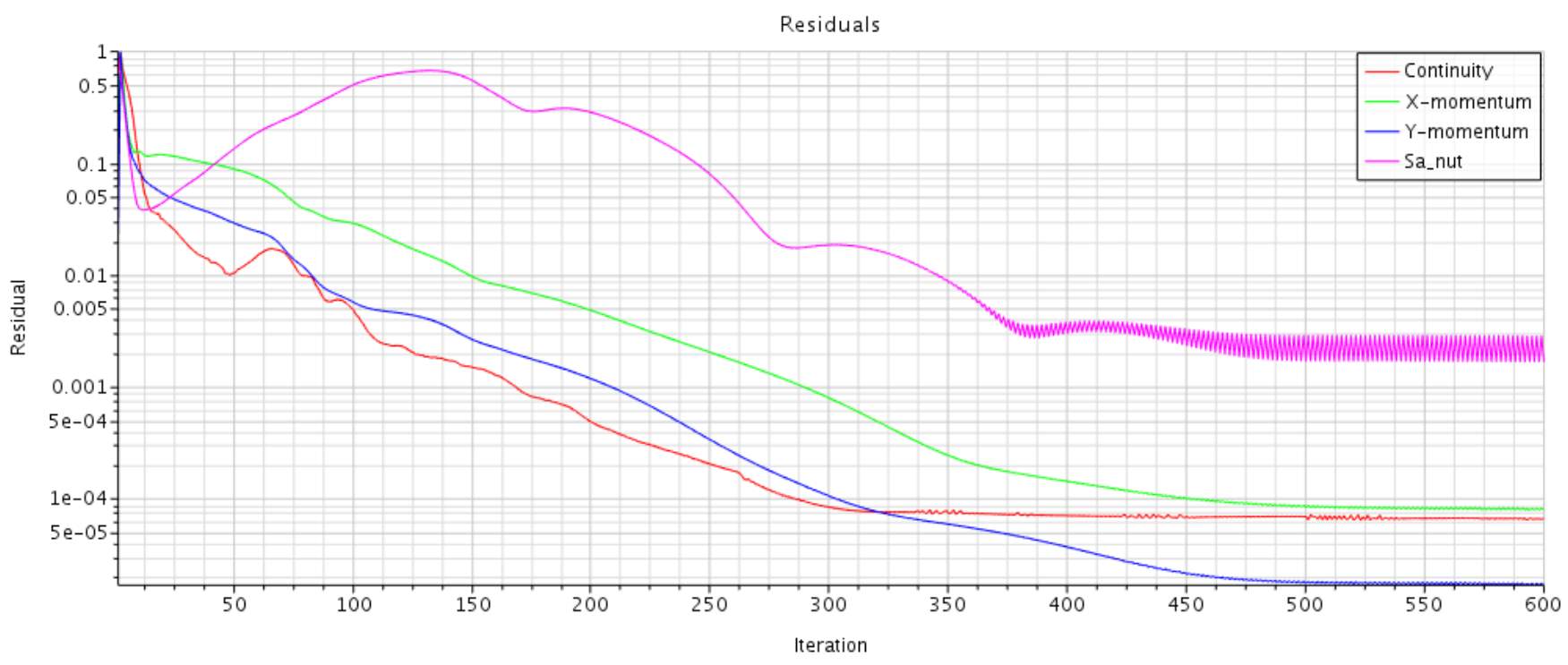
Graph 5‑1 Residuals of Benchmark Test
Once a CFD simulation is completed, a residual graph is obtained shown in Graph 5‑1. This graph shows if the simulation has converged and if the results are acceptable values to use for comparison. Typically, a solution is considered converged if there is drop in residual as the number of iterations (X-axis) increases and they eventually stabilise. The results obtained from a converged CFD simulation are perfectly acceptable to use for analysis. It is evident here that the residual quantitates have converged as they stabilise after 500 iterations. Thus, we can now obtain and compare results.
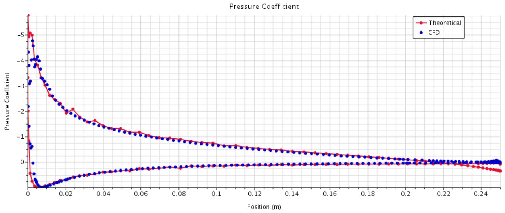
Graph 5‑2 Pressure Distribution across the NACA 0012 Aerofoil
Graph 5-2 shows the theoretical and numerical pressure distribution across the chord of my aerofoil. The graph shows that the results obtained are almost identical in comparison. This suggest that the CFD simulation was accurate and reliable. However, the lift and drag coefficients still need to be compared as they affect aerodynamic performance.
| CL | CD | |
| Theoretical (XFOIL) | 1.013 | 0.02398 |
| Numerical (CFD) | 0.9356 | 0.0336 |
Table 13 Theoretical and Numerical Benchmark Comparison
Table 13 shows the lift and drag coefficients for theoretical and numerical results for an angle of attack of 10 degrees. The results obtained are close to each other and similar. Therefore, the benchmark test proves that the numerical data is reliable and further simulation results can be used for comparison.
The results are obtained from plots of lift and drag coefficients in Star CCM+. Both the plots are shown in APPENDIX G
5.3 CFD Results
The CFD results were obtained using the setup mentioned in chapter in chapter 5.1. The test was performed for Reynolds number of 300000, corresponding to the velocity of 17.8 ms-1. The test was undertaken for angles of attack of -4 and 10 degrees. Due to the lack of time, only these conditions were simulated. However, these conditions are acceptable to for comparison and observe the icing effects.
5.3.1 Bare Wing Simulation
Firstly, the bare wing simulation were performed for the above-mentioned Reynolds number and angles of attack. This simulation is three-dimensional and all the results converged after 600 iterations. Therefore, the residual graphs are not shown here and shown in APPENDIX H. Hence, the results obtained are shown below.
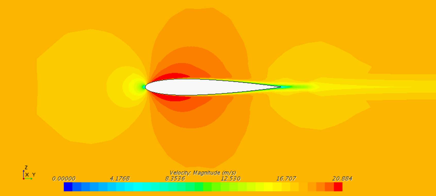 Figure 10 shows the velocity plot across a section of my wing. The velocity increases as the top of the wing, represented by the red region, and this is the same at the bottom surface. This is expected at the aerofoil is symmetrical and the velocity will be same for both, top and bottom surface of the wing. The input velocity is 17.8 ms-1 and it is increased up to 20.8 ms-1 at the top and bottom surface.
The coefficient of lift and drag were obtained using plots like that shown in chapter 5.2. The simulation is repeated for angles of attack of -4 and 10 degrees. The resulting plots are shown in APPENDIX H.
| Angle of Attack (Deg) | CL | CD |
| -4 | -0.2141 | 0.0232 |
| 0 | -0.0057 | 0.0159 |
| 10 | 0.5173 | 0.0549 |
Table 14 CFD Results (Bare Wing)
Table 14 shows results obtained from CFD simulations of bare wing. These will be compared later in chapter 6.1. The residual and coefficient plots from where the results are obtained are shown in APPENDIX H.
5.3.2 Clear Ice Simulation
An attempt was made to simulate a form of clear ice to test the iced wing in Star CCM+ although it is very difficult to simulate the exact shape to that in experimental test. However, an attempt was made and the results are shown below. The ice shape was applied at the leading edge of the wing and this was done in CATIA V5 and imported into Star CCM+.
 Shown here is the iced wing. The coloured region shows the modelled ice on the leading edge of the wing. The thickness of the simulated ice was kept the same as that in the experiment.
The above shown model was setup in Star CCM+ and the simulation was executed for angles of attack of -4 and 10 degrees. The simulation was carried out for just clear ice configuration due to shortage of time.
| Angle of Attack (Deg) | CL | CD |
| -4 | -0.2141 | 0.0232 |
| 10 | 0.5173 | 0.0549 |
Table 15 CFD Results (Clear Iced Wing)
Table 15 shows the obtained lift and drag coefficient values obtained from CFD simulations and these can be used as numerical results for comparison. The lift and drag coefficient plots with the residual convergence from Star CCM+ are shown in APPENDIX I.
6 ANALYSIS
In this chapter, the obtained results are analysed and discussed. A conclusion is drawn from the analyses and any possible improvements to the experiment and effects of ice are mentioned.
6.1 Bare Wing Data Comparison
Firstly, the experimental and theoretical results are compared to ensure that the experimental results are valid and reliable. Therefore, the bare wing results are used and lift and drag coefficients are compared.
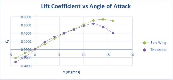
Graph 6‑1 Bare Wing Lift Comparison for Re 200000
Graph 6‑1 is plotted using values from Table 2. The graph evidently suggests that the experimental results obtained are reliable and acceptable.
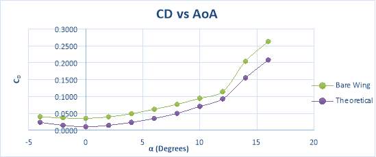
Graph 6‑2 Bare Wing Drag Comparison for Re 200000
Graph 6‑1 is plotted using values from Table 4. The results, again, are very similar as suggested in the graph. The percentage difference between experimental and theoretical result is calculated to check if the results are appropriate and the discrepancy can be explained. This is calculated using the gradients of the two graphs for both, theoretical and experimental, by drawing a trendline. The percentage difference is given by
Perecentage Difference= Difference Between Experimental TheoreticalTheoretical*100
The gradient for Graph 6-1 is calculated to be 0.0507 and 0.0426 for bare wing and theoretical respectively using MS Excel. Hence, percentage difference for lift is:
Perecentage Difference= 0.0507-0.04260.0426*100=19%
Similarly, the percentage difference for drag is calculated to be 15%.
Such a difference is acceptable in experiments performed for this project. The discrepancy could be due to various systematic and random errors. These errors include
- Interference from the Wind Tunnel: The walls of the wind tunnel and the supporting struts inside it have major interference on the flow around the wing. This is a big source of error as the distance between the tunnel walls and struts connecting to each end of the wing span is very small. Hence, it generates major interference within the flow over the wing which would result in inaccurate values.
- Instruments Errors: The speed of the wind tunnel might not be exact as it states which would affect the results. This leads to calibration errors in the instrument which would make results unreliable.
However, in general, the results obtained were acceptable and therefore the iced simulations were performed and analysed. They are analysed in the next section. The graphs shown in this section correspond to Reynolds number of 200000. The graphs obtain for other Reynolds number were very similar and generated a very similar curve to that shown in this section. Hence, they are not discussed here and are shown in APPENDIX J.
6.1.1 Bare Wing Comparison of the Three Methods
| Angle of Attack | Numerical (CFD) | Experimental | Theoretical | |||
| CL | CD | CL | CD | CL | CD | |
| -4 | -0.2141 | 0.0232 | -0.3066 | 0.0437 | -0.2980 | 0.0214 |
| 0 | -0.0057 | 0.0159 | -0.0827 | 0.0343 | 0.0000 | 0.0077 |
| 10 | 0.5173 | 0.0549 | 0.5155 | 0.0759 | 0.5594 | 0.0623 |
Table 16 Bare Wing Comparison for RE 300000
Table 16 shows the values for lift and drag coefficient for all the three methods for which the results are obtained. Here, mainly the numerical results are compared for the different simulations that were performed to other methods. The results clearly suggest that CFD model was setup accurately as the data obtained is very similar to other methods when compared. The maximum percentage difference was calculated to be 20% between numerical and theoretical results which is within the acceptable region. The discrepancy could be due to the setup in CFD. Although the setup was acceptable, it could be refined and developed which would give more accurate results. Since, CFD is numerical in nature, the mesh generated directly affects the results. Hence, refining the mesh and making it finer would improve the results. The fluid domain also has an effect as the distance between the walls and wing could cause interference in the flow.
6.2 Effects of Clear, Rime and Mixed Ice
Here, the effects of different ice accretions are compared at different Reynolds number and their effects are discussed and analysed.
The comparison of different ice accretions with clean wing and theoretical results are shown in graphs below. Three different graphs are shown which correspond to three different Reynolds numbers.
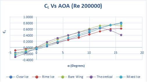
Graph 6‑3 Comparison of Lift for different Ice Simulations (RE 200000)
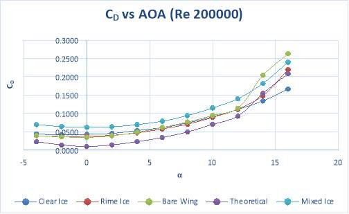
Graph 6‑4 Comparison of Drag for different Ice Simulations (RE 200000)
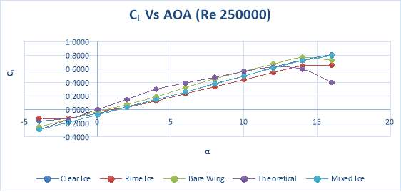
Graph 6‑5 Comparison of Lift for different Ice Simulations (RE 250000)
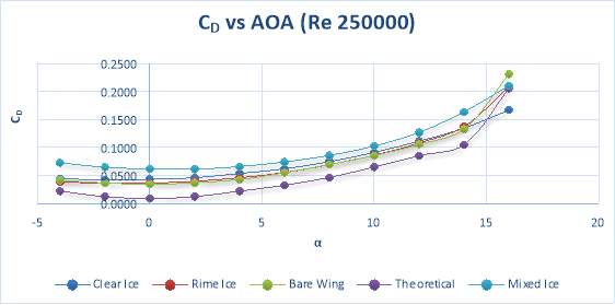
Graph 6‑6 Comparison of Drag for different Ice Simulations (RE 250000)
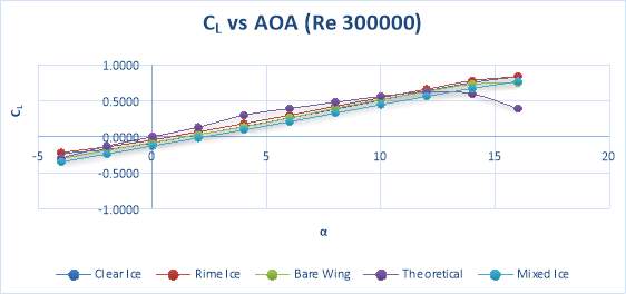
Graph 6‑7 Comparison of Lift for different Ice Simulations (RE 300000)
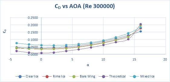
Graph 6‑8 Comparison of Drag for different Ice Simulations (RE 300000)
Above graphs show the effects of icing the aerodynamics of a wing and they were plotted using experimental and theoretical values shown chapter 3 and 4. The main effect that is evident in the graphs is the fact that lift decreases and drag increases. This consistently shown in all the graphs. This suggests, that even a small amount of ice accretion on the wing of an aircraft can have a significant impact.
The ice on the leading edge changes the shape of the aerofoil which changes the lift. The thickness of ice increases the initial chord of the wing which would increase the surface area of the wing. This change in aerofoil shape and increase in chord reduces lift. Another factor is that even a small amount of ice on a wing can drastically increase the weight of the aircraft
There is a significant increase in drag due to ice simulation on a wing. This is again due to the change in shape of the aerofoil. The roughness also plays huge part in drag increase as it interferes with flow around the aerofoil and causes turbulence which increases drag.
Cao et al., 2015 mentions that the extent of drag increase is far more than that of lift decrease. He mentions that the drag can increase by 100 – 200% when compared to the bare wing, this is in the absence of anti-icing systems. There is a significant increase in drag for the results obtained in this study, the drag, on average, is increased by 55% when compared to bare wing. This increase is for the mixed iced simulation. All the different iced configurations increased the drag and decreased the lift. Although, the mixed ice configuration increases the most amount of drag and this is expected due to it being thicker and rough compared to other comparisons. Hence, mixed iced is considered one of the most dangerous type of structural icing. The results are consistent for different velocity which prove that the results are reliable.
To summarise the effects of ice, the major effect is that of the increase in drag and decrease in lift. This significantly affects the aerodynamic efficiency of an aircraft.
6.2.1 CFD Comparison of Effects of Ice
This section highlights and compares the CFD results obtained for an iced wing. The flow around the aerofoil is compared between clean and iced to wing to further understand the effects of icing.
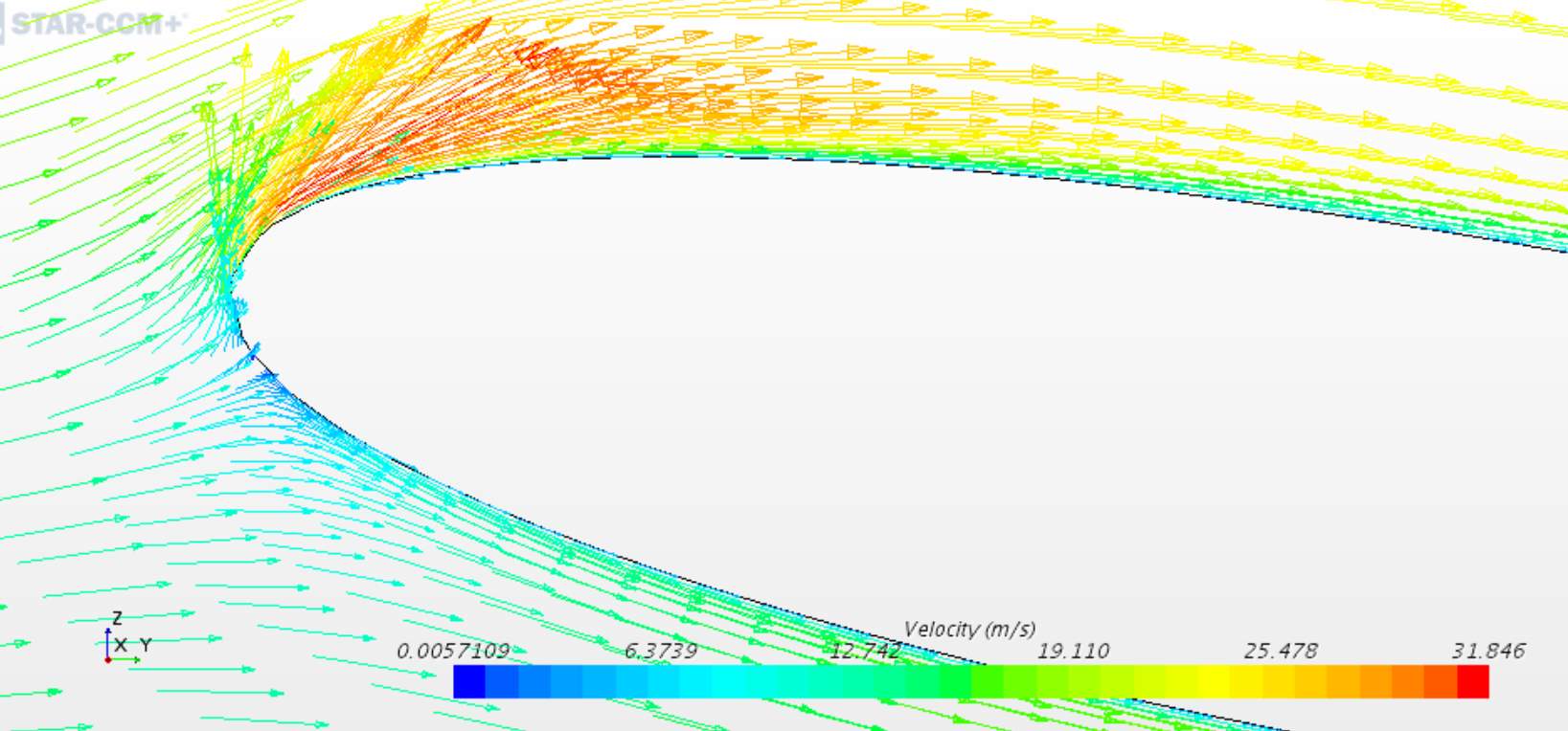
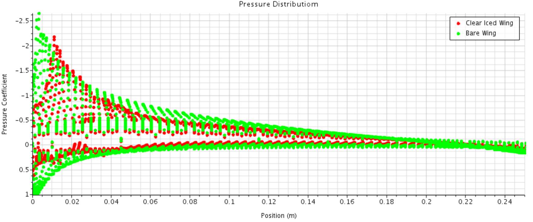
Figure 13 Flow Visualisation around Bare Wing (AOA 10)

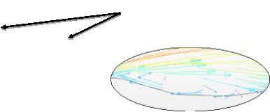
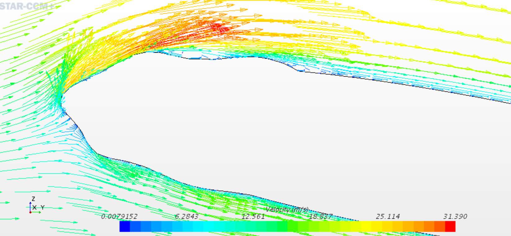
Figure 14 Flow Visualisation around Iced Wing (AOA 10)
Figures 12 and 14 show a vector plot, generated in Star CCM+ which allows us to visualise flow around an aerofoil, of bare wing and iced wing. The flow around the bare wing is smooth with no turbulence near the leading edge of the wing as expected. However, this is not the case with iced aerofoil. Firstly, Figure 14 clearly shows that the shape of the aerofoil is completely altered near the leading edge of the wing which interferes with the flow causing turbulence as it can be seen in the zoomed in picture of that section. This turbulence and eddy currents in the flow increase the drag of the wing reduces the aerodynamic performance.
Graph 6‑9 Comparison of Surface Pressure Distribution Between Iced and Bare Wing
Graph 6-9, plotted using Star CCM+, shows the pressure distribution of clean and clear iced wing for
α=10°and Reynolds number of 300000. This comparison follows on from the above analysis of flow visualisation and it provides additional results to prove the effects of ice.
The ice accretion on the leading edge of the wing has adverse effects on the surface pressure distribution of an aerofoil. As it is suggested by Graph 6-9, there is pressure drop for the iced wing due to the layer of clear ice on the leading which, as mentioned before, alters the shape of the aerofoil. This pressure suggests the lift would decrease, once again confirming the analysed effects of ice accretion. This theory of pressure distribution is supported by Da-lin and Wei-jian, 2005 as they performed a similar numerical simulation for rime ice accretion on leading edge and concluded similar effects to the ones analysed here.
This summarises the icing effects and why they have such negative effects. Hence, icing should be avoided in all cases during real flight to ensure safety.
| Angle of Attack | Numerical (CFD) | Experimental | ||
| CL | CD | CL | CD | |
| -4 | -0.2141 | 0.0232 | -0.2332 | 0.0473 |
| 10 | 0.5173 | 0.0549 | 0.4899 | 0.0912 |
Table 17 Clear Iced Wing comparison between Numerical and Experimental Results
Table 17 shows the numerical results obtained with that of experimental for clear iced wing at Reynolds number of 300000. The results obtained are very reliable as they are similar for both the methods. As mentioned before, the numerical are reliable and this is, again, confirmed here in this comparison. The lift coefficient for the two methods is almost identical and that is great achievement as modelling ice in CFD simulation is challenging and it is very difficult to model exact same shape of ice to that modelled in experimental testing. Hence, this is the numerical simulations were successful. However, the drag values are significantly higher for experimental results when compared to numerical. This is not ideal although it is expected due to high turbulence within the wind tunnel due to the walls (discussed in Chapter 6.1). The CFD simulation does not produce such high turbulence as walls of the fluid domain are further apart than the walls in the actual wind tunnel. Hence, there is the discrepancy but the results are still acceptable.
Comparing the results obtained with Broeren et al., 2011, the effects of ice are very similar. Broeren concluded that iced wing reduced the lift of the aircraft when analysing the Spanwise-Ridge ice (type of rime ice). This is what is seen in the results if this study. Hence, the effects of ice can be concluded.
6.2.2 Further Analysis and Recommendation
The results obtained in this study are acceptable and sufficient enough to observe the effects of ice on aerodynamic performance of an aircraft. However, the results can be improved and further obtained by experimenting using a different method and recording additional aerodynamic properties. An example of this is measuring pressure. The pressure distribution across the aerofoil can be measured on the top and bottom surface of wing and the difference between these pressure values could be used to calculate lift. This would provide that additional method of calculating lift which would make the results precise. Similar measurement and experiment is carried out by Broeren et al., 2011.
Another experiment could be to obtain experimental flow visualisation. A numerical flow visualisation using CFD can be obtained, as shown in Chapter 6.2.1. However, an experimental flow visualisation would show the turbulence caused by the wind tunnel which can provide better understanding of the discrepancy between results. This can be done by attaching a piece of string at various points across the surface of the wing and observing the flow they produced. This can be sketched at compared with numerical results. This would, again, increase the precision of the results and provide further understanding of the data.
There is also the possibility to analyse the effects of surface roughness due to ice accretion. Broeren et al., 2011 evaluated these effects for their wind tunnel experiment. The roundness of the surface was controlled by applying a percentage of rough materials to the surface of the airfoil. Broeren et al., 2011, used materials like glass microbeads and carborundum grains to implement roughness to their experiment. The percentage of these materials were altered to control the roughness. Such a method is very useful to implement in a study similar to this project as it allows us to observe the effects of roughness due to ice. The roughness aspect was, initially, planned to be incorporate within this study but due to the lack of time, it could not be included. However, it is a very useful method to implement in future experiment as it provides valuable insights into the effects of ice accretion.
7 CONCLUSION
To conclude, the overall project can be classed as a successful one. The aims and objectives, initially, agreed for this project were achieved. The adverse effects of ice were analysed in detail using three different methods experimental, numerical and theoretical. Enough evidence was extracted from the obtained results and analysis to conclude this study. The results were also compared with literature search where similar experiments were performed and their results were compared. This supported the analysis of this project.
Ice accretion is a phenomenon that affects both the aerodynamic performance and the flow around the wing. It majorly contributes to the formation eddy currents on the upper surface of the aerofoil downstream from the leading edge. The most adverse effects of ice accretion are reduced aerodynamic performance including a significant increase in drag and a decrease in pressure distribution across the surface of the aerofoil which leads to a serious decrease in the lift. Typically, ice accretion increases the weight of an aircraft, reduces lift, increase drag and decreases thrust. These effects were visible in this is study and appropriate analyses was performed.
REFERENCES
Airfoiltools.com. (2017). NACA 0012 AIRFOILS (n0012-il). [online] Available at: http://airfoiltools.com/airfoil/details?airfoil=n0012-il [Accessed 16 Apr. 2017].
Broeren, A., Addy, Jr., H., Bragg, M. and Busch, G. (2011). Aerodynamic Simulation of Ice Accretion on Airfoils. 1st ed. Cleveland, Ohio: NASA.
Cao, Y., Wu, Z., Su, Y. and Xu, Z. (2015). Aircraft flight characteristics in icing conditions. Progress in Aerospace Sciences, 74, pp.62-80.
Chapter 10 – ICING. (2017). 1st ed. Federal Aviation Authority.
Da-lin, Z. and Wei-jian, C. (2005). Numerical simulation of rime ice accretion process on an airfoil. Heat Transfer—Asian Research, 34(4), pp.226-234.
Disciples of Flight. (2017). Cessna 152. [online] Available at: https://disciplesofflight.com/cessna-152/ [Accessed 18 Feb. 2017].
Drela, M. (2017). XFOIL – Subsonic Airfoil Development System. [online] Web.mit.edu. Available at: http://web.mit.edu/drela/Public/web/xfoil/ [Accessed 10 Jan. 2017].
Eniscuola. (2017). The physical properties of ice – Eniscuola. [online] Available at: http://www.eniscuola.net/en/argomento/ice-and-glaciers/ice/the-physical-properties-of-ice/ [Accessed 16 Mar. 2017].
Hotwire Systems OÜ. (2017). What is polystyrene foam? | Different uses of polystyrene -. [online] Available at: http://www.hotwiresystems.com/what-is-polystyrene-eps-xps-different-uses-of-polystyrene/ [Accessed 16 Apr. 2017].
Information Manual. (1979). 1st ed. [ebook] Wichita, Kansas: Cessna Aircraft Company, p.2. Available at: http://smartaero.pl/images/stories/c152/C152-POH_80.pdf [Accessed 13 Apr. 2017].
Kemdent.co.uk. (2017). Kemdent’s Eco-friendly Modelling Wax. [online] Available at: http://www.kemdent.co.uk/new-eco-friendly-modelling-wax [Accessed 20 Nov. 2016].
Lerner, J. and Boldes, U. (2011). Wind tunnels and experimental fluid dynamics research. 1st ed. Rijeka, Croatia: InTech, pp.236-237.
Mh-aerotools.de. (2017). Airfoil and aircraft polars have been used for a long time in aeronautics. [online] Available at: http://www.mh-aerotools.de/airfoils/hdi_aoawing.htm [Accessed 13 Mar. 2017].
Smetana, F. (2001). Flight vehicle performance and aerodynamic control. Reston, Va.: American Institute of Aeronautics and Astronautics.
Warr, P. (2017). Hazards of Flight in Heavy Rain. 1st ed. smartcockpit.com.
Wind Shear. (2008). 1st ed. [ebook] Federal Aviation Administration.
BIBLIOGRAPHY
BRAGG, M. (1988). Experimental aerodynamic characteristics of an NACA 0012 airfoil with simulated glaze ice. Journal of Aircraft, 25(9), pp.849-854.
Cao, Y., Huang, J. and Yin, J. (2016). Numerical simulation of three-dimensional ice accretion on an aircraft wing. International Journal of Heat and Mass Transfer, 92, pp.34-54.
Cao, Y., Ma, C., Zhang, Q. and Sheridan, J. (2012). Numerical simulation of ice accretions on an aircraft wing. Aerospace Science and Technology, 23(1), pp.296-304.
Katz, J. and Plotkin, A. (2001). Low speed aerodynamics. 1st ed. Cambridge: Cambridge University Press.
Shin, J. and Bond, T. (2017). Experimental and Computational Ice Shapes and Resulting Drag Increase for a NACA 0012 Airfoil. 1st ed. Cleveland, Ohio: NASA.
APPENDIX A – SCREENSHOT OF XFOIL Pressure Distribution and Command Window for Reynold’s Number of 300000.
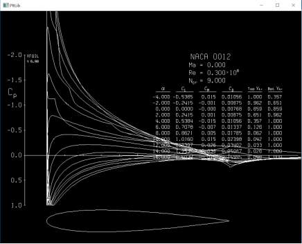
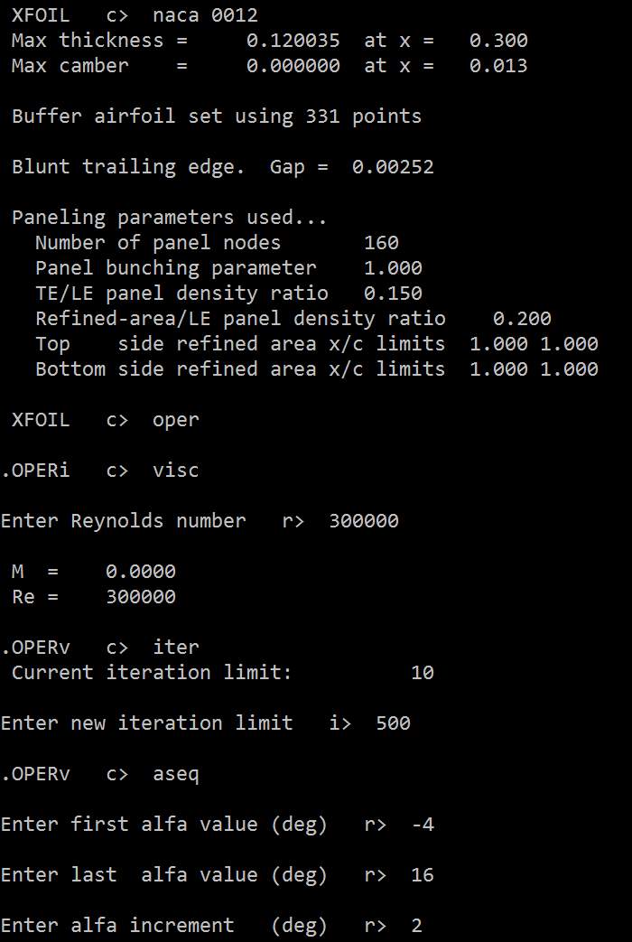
Figure 15 Screenshot of XFOIL Command Window
APPENDIX B – NACA 0012 Aerofoil Coordinates
| Airfoil surface | |
| X(mm) | Y(mm) |
| 250.0000 | 0.3150 |
| 249.8540 | 0.3355 |
| 249.4165 | 0.3968 |
| 248.6883 | 0.4985 |
| 247.6713 | 0.6399 |
| 246.3677 | 0.8201 |
| 244.7807 | 1.0380 |
| 242.9140 | 1.2921 |
| 240.7718 | 1.5810 |
| 238.3593 | 1.9027 |
| 235.6820 | 2.2554 |
| 232.7462 | 2.6371 |
| 229.5588 | 3.0456 |
| 226.1271 | 3.4786 |
| 222.4593 | 3.9338 |
| 218.5639 | 4.4088 |
| 214.4499 | 4.9013 |
| 210.1270 | 5.4087 |
| 205.6053 | 5.9286 |
| 200.8953 | 6.4584 |
| 196.0081 | 6.9957 |
| 190.9551 | 7.5379 |
| 185.7479 | 8.0824 |
| 180.3990 | 8.6265 |
| 174.9206 | 9.1675 |
| 169.3256 | 9.7027 |
| 163.6271 | 10.2294 |
| 157.8384 | 10.7445 |
| 151.9730 | 11.2451 |
| 146.0447 | 11.7281 |
| 140.0671 | 12.1905 |
| 134.0544 | 12.6290 |
| 128.0205 | 13.0405 |
| 121.9795 | 13.4217 |
| 115.9457 | 13.7692 |
| 109.9329 | 14.0800 |
| 103.9554 | 14.3508 |
| 98.0270 | 14.5786 |
| 92.1616 | 14.7605 |
| 86.3729 | 14.8937 |
| 80.6744 | 14.9757 |
| 75.0794 | 15.0043 |
| 69.6011 | 14.9776 |
| 64.2521 | 14.8939 |
| 59.0450 | 14.7520 |
| 53.9919 | 14.5512 |
| 49.1047 | 14.2910 |
| 44.3947 | 13.9714 |
| 39.8730 | 13.5929 |
| 35.5501 | 13.1563 |
| 31.4362 | 12.6628 |
| 27.5407 | 12.1142 |
| 23.8729 | 11.5122 |
| 20.4412 | 10.8593 |
| 17.2538 | 10.1578 |
| 14.3180 | 9.4104 |
| 11.6407 | 8.6198 |
| 9.2282 | 7.7890 |
| 7.0860 | 6.9207 |
| 5.2193 | 6.0177 |
| 3.6323 | 5.0825 |
| 2.3287 | 4.1177 |
| 1.3117 | 3.1253 |
| 0.5836 | 2.1072 |
| 0.1460 | 1.0651 |
| 0.0000 | 0.0000 |
| 0.1460 | -1.0651 |
| 0.5836 | -2.1072 |
| 1.3117 | -3.1253 |
| 2.3287 | -4.1177 |
| 3.6323 | -5.0825 |
| 5.2193 | -6.0177 |
| 7.0860 | -6.9207 |
| 9.2282 | -7.7890 |
| 11.6407 | -8.6198 |
| 14.3180 | -9.4104 |
| 17.2538 | -10.1578 |
| 20.4412 | -10.8593 |
| 23.8729 | -11.5122 |
| 27.5407 | -12.1142 |
| 31.4362 | -12.6628 |
| 35.5501 | -13.1563 |
| 39.8730 | -13.5929 |
| 44.3947 | -13.9714 |
| 49.1047 | -14.2910 |
| 53.9919 | -14.5512 |
| 59.0450 | -14.7520 |
| 64.2521 | -14.8939 |
| 69.6011 | -14.9776 |
| 75.0794 | -15.0043 |
| 80.6744 | -14.9757 |
| 86.3729 | -14.8937 |
| 92.1616 | -14.7605 |
| 98.0270 | -14.5786 |
| 103.9554 | -14.3508 |
| 109.9329 | -14.0800 |
| 115.9457 | -13.7692 |
| 121.9795 | -13.4217 |
| 128.0205 | -13.0405 |
| 134.0544 | -12.6290 |
| 140.0671 | -12.1905 |
| 146.0447 | -11.7281 |
| 151.9730 | -11.2451 |
| 157.8384 | -10.7445 |
| 163.6271 | -10.2294 |
| 169.3256 | -9.7027 |
| 174.9206 | -9.1675 |
| 180.3990 | -8.6265 |
| 185.7479 | -8.0824 |
| 190.9551 | -7.5379 |
| 196.0081 | -6.9957 |
| 200.8953 | -6.4584 |
| 205.6053 | -5.9286 |
| 210.1270 | -5.4087 |
| 214.4499 | -4.9013 |
| 218.5639 | -4.4088 |
| 222.4593 | -3.9338 |
| 226.1271 | -3.4786 |
| 229.5588 | -3.0456 |
| 232.7462 | -2.6371 |
| 235.6820 | -2.2554 |
| 238.3593 | -1.9027 |
| 240.7718 | -1.5810 |
| 242.9140 | -1.2921 |
| 244.7807 | -1.0380 |
| 246.3677 | -0.8201 |
| 247.6713 | -0.6399 |
| 248.6883 | -0.4985 |
| 249.4165 | -0.3968 |
| 249.8540 | -0.3355 |
| 250.0000 | -0.3150 |
APPENDIX C – EXPERIMENTAL RESULTS FOR BARE WING
| Angle of Attack | Lift (N) | Drag (N) | Average CL | Average CD | ||||||
| Test 1 | Test 2 | Test 3 | Average | Test 1 | Test 2 | Test 3 | Average | |||
| -4 | -4.9640 | -4.9820 | -4.9790 | -4.9750 | 0.8000 | 0.7838 | 0.7876 | 0.7905 | -0.2580 | 0.0415 |
| -2 | -2.8050 | -2.6520 | -2.8230 | -2.7600 | 0.7054 | 0.6851 | 0.6866 | 0.6924 | -0.1431 | 0.0366 |
| 0 | -0.5925 | -0.6051 | -0.6332 | -0.6103 | 0.6570 | 0.6655 | 0.6525 | 0.6583 | -0.0316 | 0.0341 |
| 2 | 1.4080 | 1.3950 | 1.3580 | 1.3870 | 0.7139 | 0.7195 | 0.7019 | 0.7118 | 0.0719 | 0.0370 |
| 4 | 3.6130 | 3.6480 | 3.6150 | 3.6253 | 0.8220 | 0.8296 | 0.8097 | 0.8204 | 0.1880 | 0.0426 |
| 6 | 6.2870 | 6.1650 | 6.2190 | 6.2237 | 1.0580 | 1.0650 | 1.0450 | 1.0560 | 0.3227 | 0.0549 |
| 8 | 8.8030 | 8.6470 | 8.6710 | 8.7070 | 1.3390 | 1.3470 | 1.3150 | 1.3337 | 0.4515 | 0.0694 |
| 10 | 10.8500 | 10.8900 | 10.8200 | 10.8533 | 1.6480 | 1.6250 | 1.6520 | 1.6417 | 0.5628 | 0.0855 |
| 12 | 12.8400 | 12.8700 | 12.8100 | 12.8400 | 2.0340 | 2.0450 | 2.0430 | 2.0407 | 0.6658 | 0.1055 |
| 14 | 14.8200 | 14.8600 | 14.7000 | 14.7933 | 2.5590 | 2.5710 | 2.5590 | 2.5630 | 0.7671 | 0.1327 |
| 16 | 13.7300 | 14.2600 | 13.7300 | 13.9067 | 4.4490 | 4.4430 | 4.4340 | 4.4420 | 0.7211 | 0.2307 |
| Angle of Attack | Lift (N) | Drag (N) | Average CL | Average CD | ||||||
| Test 1 | Test 2 | Test 3 | Average | Test 1 | Test 2 | Test 3 | Average | |||
| -4 | -8.5070 | -8.5800 | -8.5690 | -8.5520 | 1.2190 | 1.2220 | 1.2310 | 1.2240 | -0.3066 | 0.0437 |
| -2 | -5.2810 | -5.2950 | -5.2930 | -5.2897 | 1.0340 | 1.0400 | 1.0500 | 1.0413 | -0.1896 | 0.0371 |
| 0 | -2.3170 | -2.3040 | -2.2970 | -2.3060 | 0.9577 | 0.9591 | 0.9597 | 0.9588 | -0.0827 | 0.0343 |
| 2 | 0.7602 | 0.8144 | 0.8331 | 0.8026 | 0.9630 | 0.9841 | 0.9870 | 0.9780 | 0.0288 | 0.0345 |
| 4 | 3.7010 | 3.8740 | 3.7140 | 3.7630 | 1.0750 | 1.0940 | 1.0820 | 1.0837 | 0.1349 | 0.0385 |
| 6 | 7.1260 | 7.3120 | 7.3020 | 7.2467 | 1.3310 | 1.3620 | 1.3400 | 1.3443 | 0.2598 | 0.0477 |
| 8 | 10.8400 | 11.1300 | 10.9700 | 10.9800 | 1.7000 | 1.7440 | 1.7230 | 1.7223 | 0.3936 | 0.0609 |
| 10 | 14.2900 | 14.5300 | 14.3200 | 14.3800 | 2.1170 | 2.1780 | 2.1430 | 2.1460 | 0.5155 | 0.0759 |
| 12 | 17.2900 | 17.5400 | 17.4100 | 17.4133 | 2.6430 | 2.6790 | 2.6680 | 2.6633 | 0.6242 | 0.0947 |
| 14 | 20.2700 | 20.4500 | 20.3400 | 20.3533 | 3.2800 | 3.3510 | 3.3040 | 3.3117 | 0.7296 | 0.1176 |
| 16 | 20.7900 | 20.6100 | 20.6700 | 20.6900 | 5.4840 | 5.4320 | 5.4300 | 5.4487 | 0.7417 | 0.1966 |
APPENDIX D – RIME ICE EXPERIMENTAL RESULTS
| Angle of Attack | Lift (N) | Drag (N) | Average CL | Average CD | ||||||
| Test 1 | Test 2 | Test 3 | Average | Test 1 | Test 2 | Test 3 | Average | |||
| -4 | -2.1410 | -0.5636 | -0.7207 | -1.1418 | 0.5004 | 0.4868 | 0.4781 | 0.4884 | -0.0931 | 0.0398 |
| -2 | -2.0290 | 0.7354 | -0.5546 | -0.6161 | 0.4599 | 0.4628 | 0.4546 | 0.4591 | -0.0503 | 0.0374 |
| 0 | -1.5260 | 1.6230 | -0.2411 | -0.0480 | 0.4752 | 0.4584 | 0.4634 | 0.4657 | -0.0039 | 0.0380 |
| 2 | -0.9997 | 3.6280 | 0.3396 | 0.9893 | 0.4831 | 0.5006 | 0.5092 | 0.4976 | 0.0807 | 0.0406 |
| 4 | 0.7786 | 4.9660 | 0.7049 | 2.1498 | 0.5766 | 0.5910 | 0.5777 | 0.5818 | 0.1754 | 0.0475 |
| 6 | 1.8070 | 6.0720 | 1.3290 | 3.0693 | 0.7092 | 0.7098 | 0.7189 | 0.7126 | 0.2504 | 0.0581 |
| 8 | 2.7640 | 7.1390 | 1.9730 | 3.9587 | 0.8762 | 0.8788 | 0.8540 | 0.8697 | 0.3229 | 0.0709 |
| 10 | 4.2200 | 8.0050 | 3.3830 | 5.2027 | 1.0900 | 1.1110 | 1.0970 | 1.0993 | 0.4244 | 0.0897 |
| 12 | 5.2240 | 8.3980 | 5.6820 | 6.4347 | 1.3720 | 1.3880 | 1.3640 | 1.3747 | 0.5249 | 0.1121 |
| 14 | 6.5890 | 8.6700 | 6.7930 | 7.3507 | 1.8190 | 1.8360 | 1.8160 | 1.8237 | 0.5996 | 0.1488 |
| 16 | 6.9860 | 8.2120 | 7.6000 | 7.5993 | 2.7340 | 2.7140 | 2.6500 | 2.6993 | 0.6199 | 0.2202 |
| Angle of Attack | Lift (N) | Drag (N) | Average CL | Average CD | ||||||
| Test 1 | Test 2 | Test 3 | Average | Test 1 | Test 2 | Test 3 | Average | |||
| -4 | -2.9840 | -2.3540 | -2.3160 | -2.5513 | 0.7368 | 0.7511 | 0.7505 | 0.7461 | -0.1323 | 0.0387 |
| -2 | -2.6870 | -2.6870 | -2.0820 | -2.4853 | 0.6810 | 0.7025 | 0.6884 | 0.6906 | -0.1289 | 0.0358 |
| 0 | -2.0520 | 1.5150 | -1.4010 | -0.6460 | 0.6934 | 0.7003 | 0.7056 | 0.6998 | -0.0335 | 0.0363 |
| 2 | -1.2880 | 3.8150 | -0.6796 | 0.6158 | 0.7643 | 0.7605 | 0.7684 | 0.7644 | 0.0319 | 0.0396 |
| 4 | 1.1040 | 5.9810 | 0.1458 | 2.4103 | 0.8683 | 0.9091 | 0.8775 | 0.8850 | 0.1250 | 0.0459 |
| 6 | 3.3260 | 8.3230 | 1.8500 | 4.4997 | 1.0560 | 1.0800 | 1.0570 | 1.0643 | 0.2333 | 0.0552 |
| 8 | 5.0480 | 10.5300 | 3.7450 | 6.4410 | 1.3270 | 1.3410 | 1.3400 | 1.3360 | 0.3340 | 0.0693 |
| 10 | 7.0680 | 12.1700 | 6.0790 | 8.4390 | 1.6480 | 1.6850 | 1.6430 | 1.6587 | 0.4376 | 0.0860 |
| 12 | 9.1400 | 13.3300 | 8.9400 | 10.4700 | 2.0610 | 2.1060 | 2.0760 | 2.0810 | 0.5429 | 0.1079 |
| 14 | 11.9500 | 13.8900 | 11.2800 | 12.3733 | 2.6220 | 2.6780 | 2.6380 | 2.6460 | 0.6416 | 0.1372 |
| 16 | 12.3000 | 12.6800 | 12.7900 | 12.5900 | 4.0020 | 4.0720 | 4.0180 | 4.0307 | 0.6528 | 0.2090 |
| Angle of Attack | Lift (N) | Drag (N) | Average CL | Average CD | ||||||
| Test 1 | Test 2 | Test 3 | Average | Test 1 | Test 2 | Test 3 | Average | |||
| -4 | -6.8290 | -5.5240 | -5.5530 | -5.9687 | 1.1290 | 1.1170 | 1.1020 | 1.1160 | -0.2214 | 0.0414 |
| -2 | -4.2310 | -2.4400 | -4.6750 | -3.7820 | 0.9887 | 0.9954 | 1.0060 | 0.9967 | -0.1403 | 0.0370 |
| 0 | -1.1850 | 0.7615 | -3.3350 | -1.2528 | 0.9909 | 0.9587 | 0.9738 | 0.9745 | -0.0465 | 0.0361 |
| 2 | 1.9080 | 3.3650 | 0.1849 | 1.8193 | 1.0340 | 1.0080 | 1.0170 | 1.0197 | 0.0675 | 0.0378 |
| 4 | 4.9180 | 6.3850 | 3.3410 | 4.8813 | 1.1610 | 1.1580 | 1.1530 | 1.1573 | 0.1810 | 0.0429 |
| 6 | 8.1270 | 9.7820 | 6.1930 | 8.0340 | 1.3700 | 1.3840 | 1.3720 | 1.3753 | 0.2979 | 0.0510 |
| 8 | 11.2500 | 13.0300 | 9.8640 | 11.3813 | 1.6920 | 1.7030 | 1.6950 | 1.6967 | 0.4221 | 0.0629 |
| 10 | 14.7000 | 16.1700 | 12.9700 | 14.6133 | 2.1380 | 2.1250 | 2.1050 | 2.1227 | 0.5420 | 0.0787 |
| 12 | 16.8800 | 19.5100 | 16.9000 | 17.7633 | 2.6500 | 2.6570 | 2.6310 | 2.6460 | 0.6588 | 0.0981 |
| 14 | 21.2200 | 21.7300 | 19.9200 | 20.9567 | 3.3120 | 3.3200 | 3.2750 | 3.3023 | 0.7772 | 0.1225 |
| 16 | 22.1900 | 23.1200 | 22.0100 | 22.4400 | 4.8100 | 4.5990 | 4.7830 | 4.7307 | 0.8322 | 0.1754 |
APPENDIX E – CLEAR ICE EXPERIMENTAL RESULTS
| Angle of Attack | Lift (N) | Drag (N) | Average CL | Average CD | ||||||
| Test 1 | Test 2 | Test 3 | Average | Test 1 | Test 2 | Test 3 | Average | |||
| -4 | -1.2560 | -0.9194 | -0.9076 | -1.0277 | 0.5747 | 0.5774 | 0.5887 | 0.5803 | -0.0914 | 0.0473 |
| -2 | -0.9166 | 0.6120 | -0.5310 | -0.2785 | 0.5483 | 0.5674 | 0.5634 | 0.5597 | -0.0248 | 0.0457 |
| 0 | -0.5167 | 2.1600 | -0.1918 | 0.4838 | 0.5573 | 0.5524 | 0.5593 | 0.5563 | 0.0430 | 0.0454 |
| 2 | 0.2770 | 3.1840 | 0.3306 | 1.2639 | 0.6013 | 0.6034 | 0.6041 | 0.6029 | 0.1124 | 0.0492 |
| 4 | 1.6580 | 4.8586 | 1.1850 | 2.5672 | 0.6869 | 0.6912 | 0.6934 | 0.6905 | 0.2283 | 0.0563 |
| 6 | 2.6190 | 5.4010 | 2.6080 | 3.5427 | 0.8016 | 0.8318 | 0.8147 | 0.8160 | 0.3151 | 0.0666 |
| 8 | 4.0010 | 7.2330 | 4.2890 | 5.1743 | 0.9555 | 0.9812 | 0.9941 | 0.9769 | 0.4602 | 0.0797 |
| 10 | 5.8140 | 8.9490 | 5.8480 | 6.8703 | 1.1870 | 1.1860 | 1.1900 | 1.1877 | 0.6111 | 0.0969 |
| 12 | 7.3700 | 9.3280 | 7.1350 | 7.9443 | 1.4460 | 1.4520 | 1.4370 | 1.4450 | 0.7066 | 0.1179 |
| 14 | 8.6610 | 9.7870 | 8.9160 | 9.1213 | 1.7320 | 1.7490 | 1.7340 | 1.7383 | 0.8113 | 0.1418 |
| 16 | 10.0200 | 9.9760 | 10.0300 | 10.0087 | 2.1060 | 2.1000 | 2.1090 | 2.1050 | 0.8902 | 0.1717 |
| Angle of Attack | Lift (N) | Drag (N) | Average CL | Average CD | ||||||
| Test 1 | Test 2 | Test 3 | Average | Test 1 | Test 2 | Test 3 | Average | |||
| -4 | -3.9030 | -3.0380 | -3.0550 | -3.3320 | 0.8430 | 0.8631 | 0.8624 | 0.8562 | -0.1728 | 0.0444 |
| -2 | -3.7760 | -1.2090 | -2.5620 | -2.5157 | 0.8001 | 0.8117 | 0.8057 | 0.8058 | -0.1304 | 0.0418 |
| 0 | -2.3790 | 0.9423 | -1.9290 | -1.1219 | 0.8290 | 0.8337 | 0.8405 | 0.8344 | -0.0582 | 0.0433 |
| 2 | -0.3278 | 3.2840 | -0.6869 | 0.7564 | 0.8744 | 0.8916 | 0.8890 | 0.8850 | 0.0392 | 0.0459 |
| 4 | 1.8610 | 5.3790 | 1.3380 | 2.8593 | 0.9860 | 1.1014 | 1.0120 | 1.0331 | 0.1483 | 0.0536 |
| 6 | 3.6410 | 7.6020 | 3.6020 | 4.9483 | 1.1800 | 1.1970 | 1.2010 | 1.1927 | 0.2566 | 0.0618 |
| 8 | 6.5770 | 9.6900 | 5.8180 | 7.3617 | 1.4210 | 1.4520 | 1.4440 | 1.4390 | 0.3817 | 0.0746 |
| 10 | 8.2640 | 11.9000 | 8.1790 | 9.4477 | 1.7380 | 1.7670 | 1.7720 | 1.7590 | 0.4899 | 0.0912 |
| 12 | 11.0800 | 14.2400 | 10.5700 | 11.9633 | 2.1260 | 2.1590 | 2.1440 | 2.1430 | 0.6203 | 0.1111 |
| 14 | 13.3800 | 15.4700 | 13.2100 | 14.0200 | 2.5870 | 2.5930 | 2.5960 | 2.5920 | 0.7270 | 0.1344 |
| 16 | 15.6200 | 15.6700 | 15.4900 | 15.5933 | 3.1600 | 3.1630 | 3.3190 | 3.2140 | 0.8085 | 0.1667 |
| Angle of Attack | Lift (N) | Drag (N) | Average CL | Average CD | ||||||
| Test 1 | Test 2 | Test 3 | Average | Test 1 | Test 2 | Test 3 | Average | |||
| -4 | -6.4590 | -6.0770 | -6.3280 | -6.2880 | 1.2780 | 1.2780 | 1.2720 | 1.2760 | -0.2332 | 0.0473 |
| -2 | -5.5910 | -3.4190 | -5.5040 | -4.8380 | 1.1740 | 1.1680 | 1.1740 | 1.1720 | -0.1794 | 0.0435 |
| 0 | -3.3280 | -0.4092 | -3.2370 | -2.3247 | 1.1510 | 1.1690 | 1.1550 | 1.1583 | -0.0862 | 0.0430 |
| 2 | -0.5131 | 2.9030 | -0.1352 | 0.7516 | 1.2050 | 1.2230 | 1.2410 | 1.2230 | 0.0279 | 0.0454 |
| 4 | 2.7520 | 5.8460 | 2.7270 | 3.7750 | 1.3480 | 1.3670 | 1.3710 | 1.3620 | 0.1400 | 0.0505 |
| 6 | 5.9060 | 8.8770 | 6.2910 | 7.0247 | 1.5790 | 1.5990 | 1.6180 | 1.5987 | 0.2605 | 0.0593 |
| 8 | 9.2420 | 12.1000 | 9.5170 | 10.2863 | 1.8900 | 1.9410 | 1.9240 | 1.9183 | 0.3815 | 0.0711 |
| 10 | 12.6700 | 15.3000 | 13.1900 | 13.7200 | 2.3140 | 2.3740 | 2.3530 | 2.3470 | 0.5088 | 0.0870 |
| 12 | 16.1100 | 18.4300 | 16.6700 | 17.0700 | 2.8230 | 2.9000 | 2.8660 | 2.8630 | 0.6331 | 0.1062 |
| 14 | 19.4300 | 21.6600 | 19.6800 | 20.2567 | 3.4320 | 3.4870 | 3.4870 | 3.4687 | 0.7512 | 0.1286 |
| 16 | 22.3500 | 22.4700 | 22.6100 | 22.4767 | 4.1650 | 4.1760 | 4.1930 | 4.1780 | 0.8336 | 0.1549 |
APPENDIX F – MIXED ICE EXPERIMENTAL RESULTS
| Angle of Attack | Lift (N) | Drag (N) | Average CL | Average CD | ||||||
| Test 1 | Test 2 | Test 3 | Average | Test 1 | Test 2 | Test 3 | Average | |||
| -4 | -2.9420 | -2.9860 | -2.9540 | -2.9607 | 0.8581 | 0.8669 | 0.8763 | 0.8671 | -0.2415 | 0.0700 |
| -2 | -1.7670 | -1.6080 | -1.6800 | -1.6850 | 0.7909 | 0.8035 | 0.8103 | 0.8016 | -0.1374 | 0.0645 |
| 0 | -0.3429 | -0.2952 | -0.3030 | -0.3137 | 0.7683 | 0.7976 | 0.7859 | 0.7839 | -0.0256 | 0.0627 |
| 2 | 0.9341 | 1.1190 | 1.0230 | 1.0254 | 0.7853 | 0.7962 | 0.7859 | 0.7891 | 0.0836 | 0.0641 |
| 4 | 2.3640 | 2.4250 | 2.2970 | 2.3620 | 0.8572 | 0.8948 | 0.8766 | 0.8762 | 0.1927 | 0.0699 |
| 6 | 3.7160 | 3.8630 | 3.8440 | 3.8077 | 0.9712 | 0.9929 | 0.9862 | 0.9834 | 0.3106 | 0.0792 |
| 8 | 5.1160 | 5.2160 | 5.1990 | 5.1770 | 1.1570 | 1.1680 | 1.1690 | 1.1647 | 0.4223 | 0.0944 |
| 10 | 6.4800 | 6.6810 | 6.6110 | 6.5907 | 1.4130 | 1.4510 | 1.4220 | 1.4287 | 0.5376 | 0.1153 |
| 12 | 7.8970 | 8.1460 | 7.9250 | 7.9893 | 1.7190 | 1.7530 | 1.7460 | 1.7393 | 0.6517 | 0.1402 |
| 14 | 8.8300 | 8.9970 | 9.1840 | 9.0037 | 2.2330 | 2.2720 | 2.3450 | 2.2833 | 0.7344 | 0.1821 |
| 16 | 9.3170 | 9.4340 | 9.6920 | 9.4810 | 2.9420 | 2.9620 | 2.9940 | 2.9660 | 0.7734 | 0.2400 |
Table 26 Wind Tunnel Data for RE 200000 (Mixed Iced Wing)
| Angle of Attack | Lift (N) | Drag (N) | Average CL | Average CD | ||||||
| Test 1 | Test 2 | Test 3 | Average | Test 1 | Test 2 | Test 3 | Average | |||
| -4 | -5.6880 | -5.7290 | -5.7910 | -5.7360 | 1.3990 | 1.4030 | 1.4040 | 1.4020 | -0.2974 | 0.0725 |
| -2 | -3.7130 | -3.5060 | -3.7070 | -3.6420 | 1.2470 | 1.2660 | 1.2680 | 1.2603 | -0.1888 | 0.0647 |
| 0 | -1.6170 | -1.5290 | -1.5310 | -1.5590 | 1.1870 | 1.2000 | 1.1830 | 1.1900 | -0.0808 | 0.0615 |
| 2 | 0.6014 | 0.7187 | 0.5562 | 0.6254 | 1.1790 | 1.2130 | 1.1980 | 1.1967 | 0.0324 | 0.0611 |
| 4 | 2.6680 | 2.8860 | 2.7180 | 2.7573 | 1.2700 | 1.3020 | 1.2790 | 1.2837 | 0.1430 | 0.0659 |
| 6 | 4.8810 | 5.0550 | 4.9270 | 4.9543 | 1.4270 | 1.4460 | 1.4350 | 1.4360 | 0.2569 | 0.0740 |
| 8 | 7.1190 | 7.3930 | 7.1510 | 7.2210 | 1.6550 | 1.6940 | 1.6600 | 1.6697 | 0.3744 | 0.0858 |
| 10 | 9.4290 | 9.6950 | 9.4620 | 9.5287 | 1.9770 | 2.0380 | 1.9920 | 2.0023 | 0.4941 | 0.1025 |
| 12 | 11.6000 | 11.9200 | 11.6300 | 11.7167 | 2.4470 | 2.5160 | 2.5080 | 2.4903 | 0.6075 | 0.1269 |
| 14 | 13.9000 | 13.9500 | 13.6900 | 13.8467 | 3.1570 | 3.1470 | 3.1610 | 3.1550 | 0.7180 | 0.1637 |
| 16 | 15.2500 | 15.4100 | 15.1600 | 15.2733 | 4.0550 | 4.0720 | 3.9700 | 4.0323 | 0.7919 | 0.2103 |
Table 27 Wind Tunnel Data for RE 250000 (Mixed Iced Wing)
| Angle of Attack | Lift (N) | Drag (N) | Average CL | Average CD | ||||||
| Test 1 | Test 2 | Test 3 | Average | Test 1 | Test 2 | Test 3 | Average | |||
| -4 | -9.9180 | -9.7140 | -9.7980 | -9.8100 | 2.1090 | 2.0980 | 2.1140 | 2.1070 | -0.3517 | 0.0756 |
| -2 | -6.8180 | -6.5890 | -6.7390 | -6.7153 | 1.8560 | 1.8590 | 1.8580 | 1.8577 | -0.2407 | 0.0665 |
| 0 | -3.6530 | -3.4920 | -3.5800 | -3.5750 | 1.7170 | 1.7000 | 1.7210 | 1.7127 | -0.1282 | 0.0615 |
| 2 | -0.6043 | -0.3115 | -0.5933 | -0.5030 | 1.6720 | 1.6900 | 1.6740 | 1.6787 | -0.0180 | 0.0599 |
| 4 | 2.5570 | 2.7200 | 2.6060 | 2.6277 | 1.7290 | 1.7220 | 1.7260 | 1.7257 | 0.0942 | 0.0620 |
| 6 | 5.7820 | 5.9570 | 5.7460 | 5.8283 | 1.9100 | 1.9140 | 1.9110 | 1.9117 | 0.2089 | 0.0685 |
| 8 | 9.0300 | 9.1850 | 8.9630 | 9.0593 | 2.2010 | 2.2180 | 2.1880 | 2.2023 | 0.3247 | 0.0789 |
| 10 | 12.3500 | 12.5400 | 12.3000 | 12.3967 | 2.6110 | 2.6290 | 2.5960 | 2.6120 | 0.4444 | 0.0936 |
| 12 | 15.5000 | 15.6600 | 15.5300 | 15.5633 | 3.2030 | 3.2280 | 3.1800 | 3.2037 | 0.5579 | 0.1148 |
| 14 | 18.7700 | 18.7500 | 18.5800 | 18.7000 | 3.9660 | 4.0050 | 3.9960 | 3.9890 | 0.6703 | 0.1422 |
| 16 | 21.4000 | 21.5500 | 21.2300 | 21.3933 | 5.0530 | 4.9850 | 4.9930 | 5.0103 | 0.7669 | 0.1811 |
Table 28 Wind Tunnel Data for RE 300000 (Mixed Iced Wing)
APPENDIX G – CFD BENCHMARK LIFT AND DRAG COEFFICIENT PLOTS
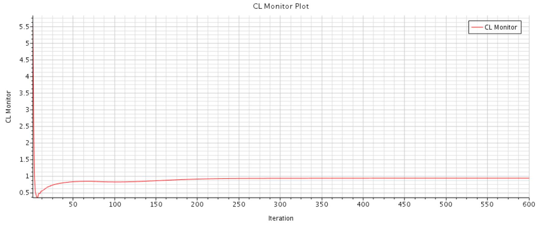
Figure 16 CL Plot for CFD Benchmark Test (AOA 10)
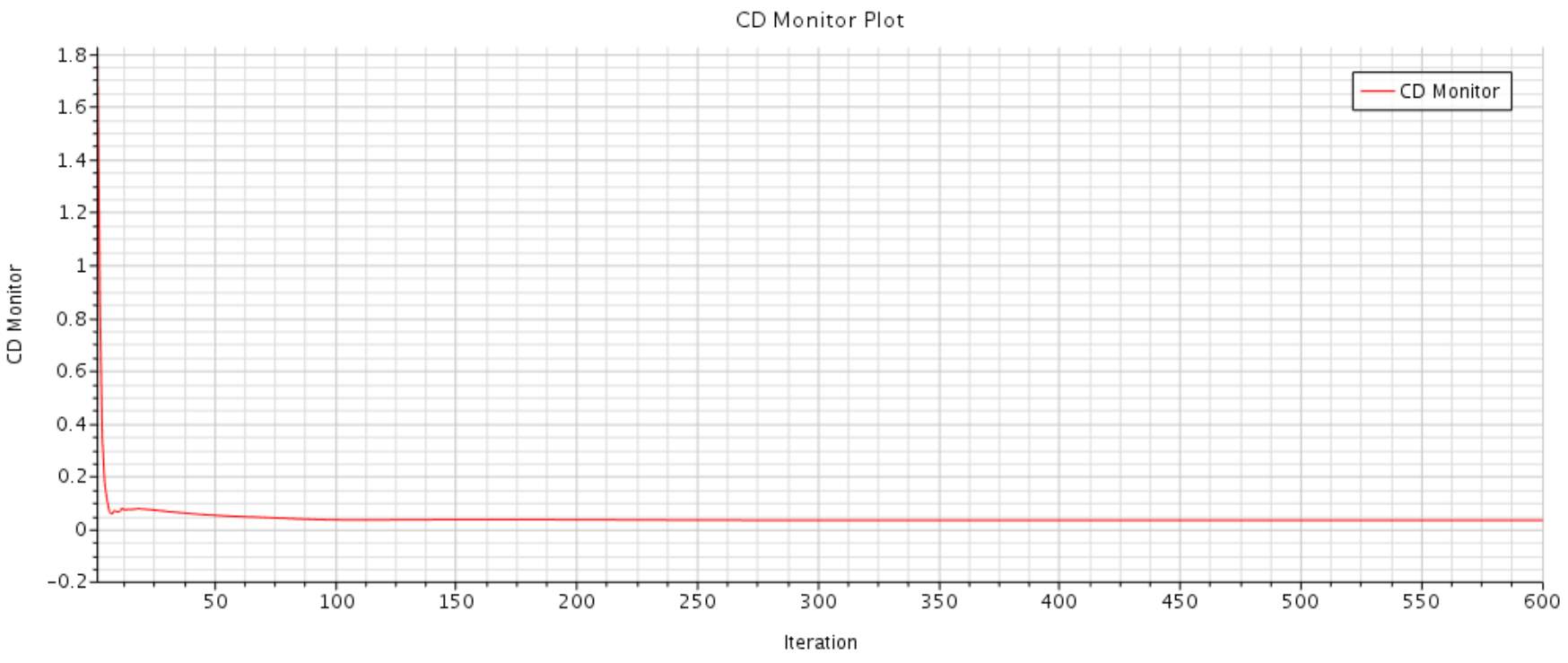
Figure 17 CD Plot for CFD Benchmark Test (AOA 10)
APPENDIX H – CFD PLOTS
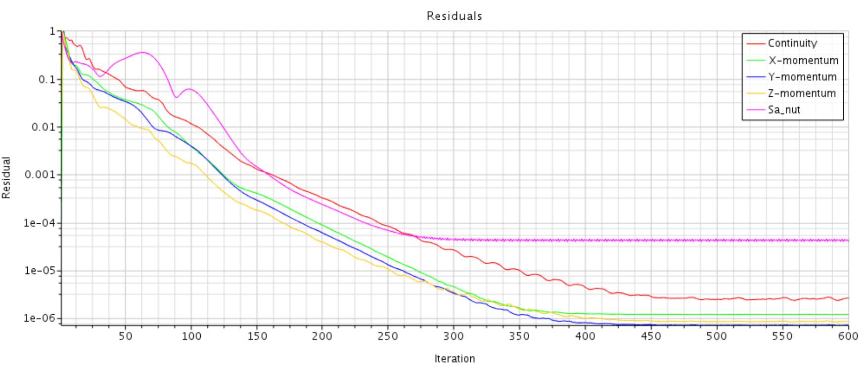
Figure 18 Residual for Bare Wing simulation AOA of 0
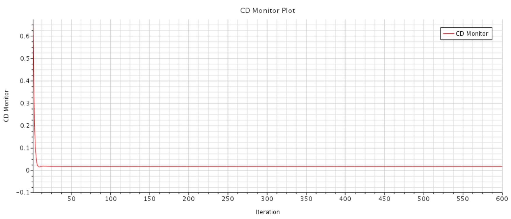
Figure 19 CL Plot for Bare Wing simulation AOA of 0
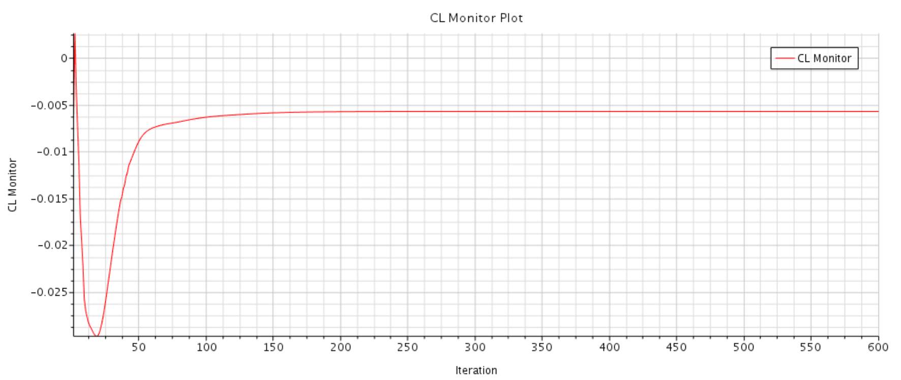
Figure 20 CD Plot for Bare Wing simulation AOA of 0
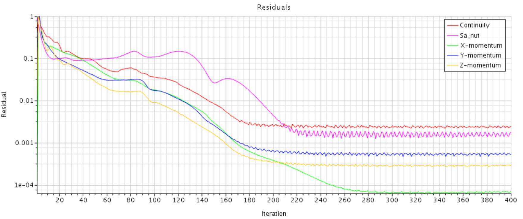
Figure 21 Residual for Bare Wing simulation AOA of -4
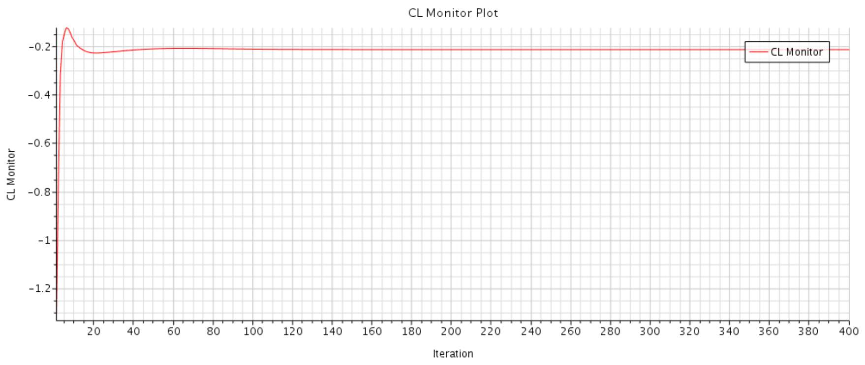
Figure 22 CL Plot for Bare Wing simulation AOA of -4
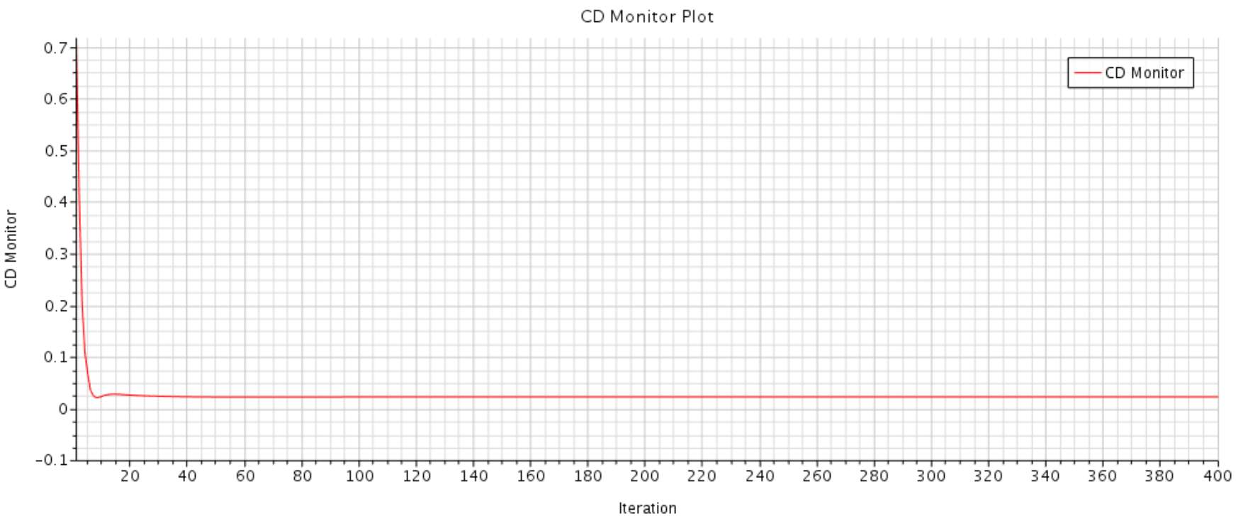
Figure 23 CD Plot for Bare Wing simulation AOA of -4
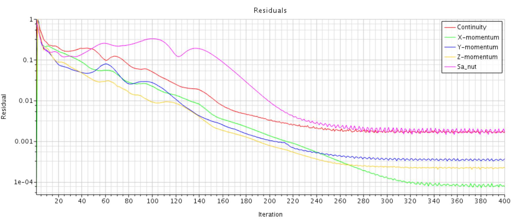
Figure 24 Residual for Bare Wing simulation AOA of 10
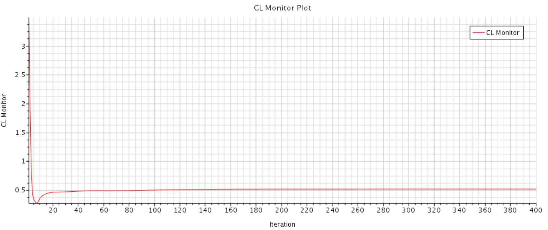
Figure 25 CL Plot for Bare Wing simulation AOA of 10
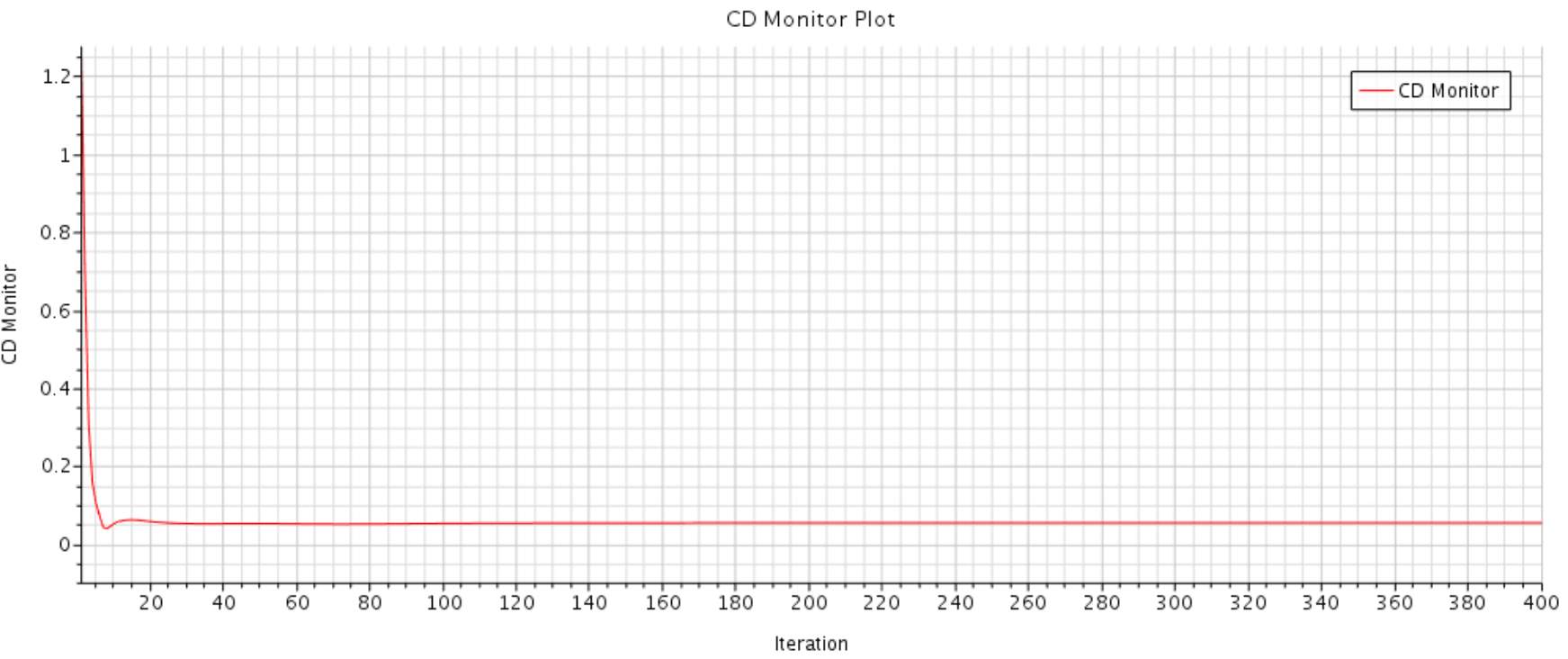
Figure 26 CD Plot for Bare Wing simulation AOA of 10
APPENDIX I – CFD PLOTS FOR ICED WING
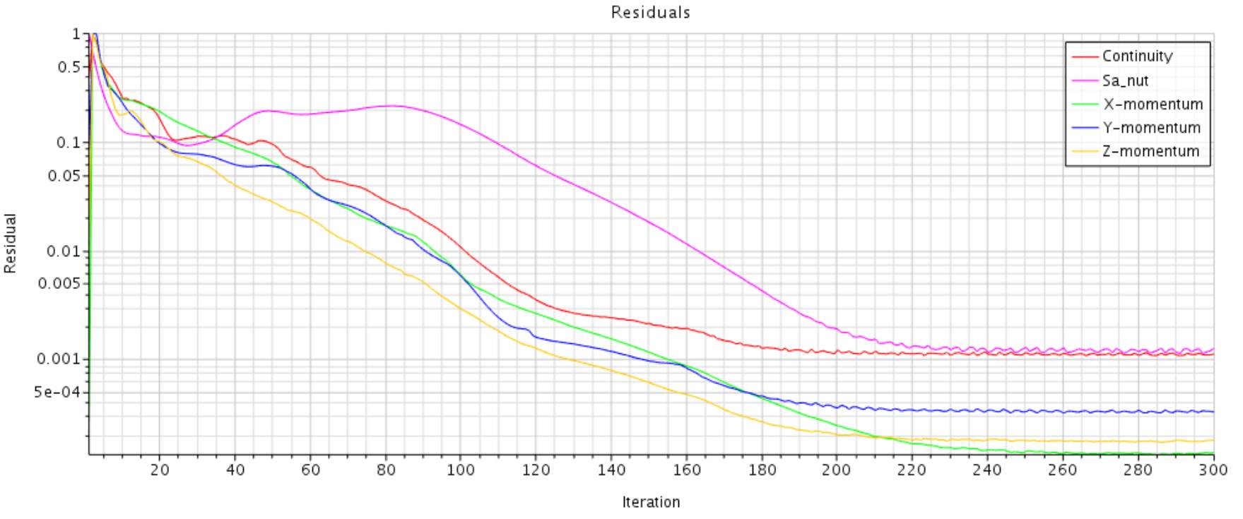
Figure 27 Residual for Clear Iced Wing simulation, AOA of -4
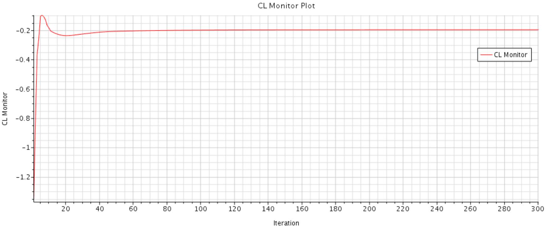
Figure 28 CL Plot for Clear Iced Wing simulation, AOA of -4
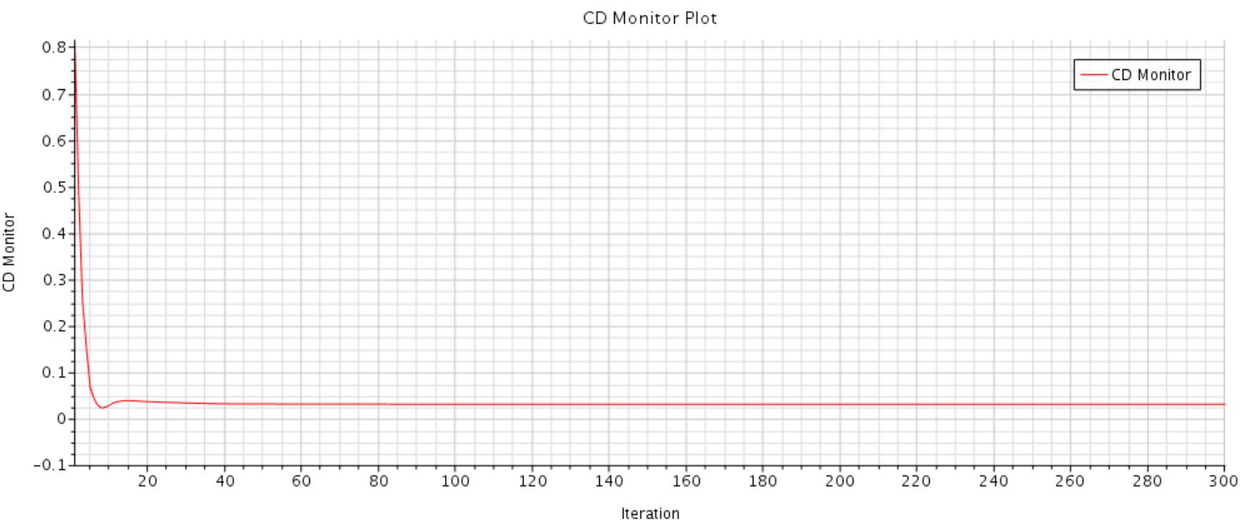
Figure 29 CD Plot for Clear Iced Wing simulation, AOA of -4
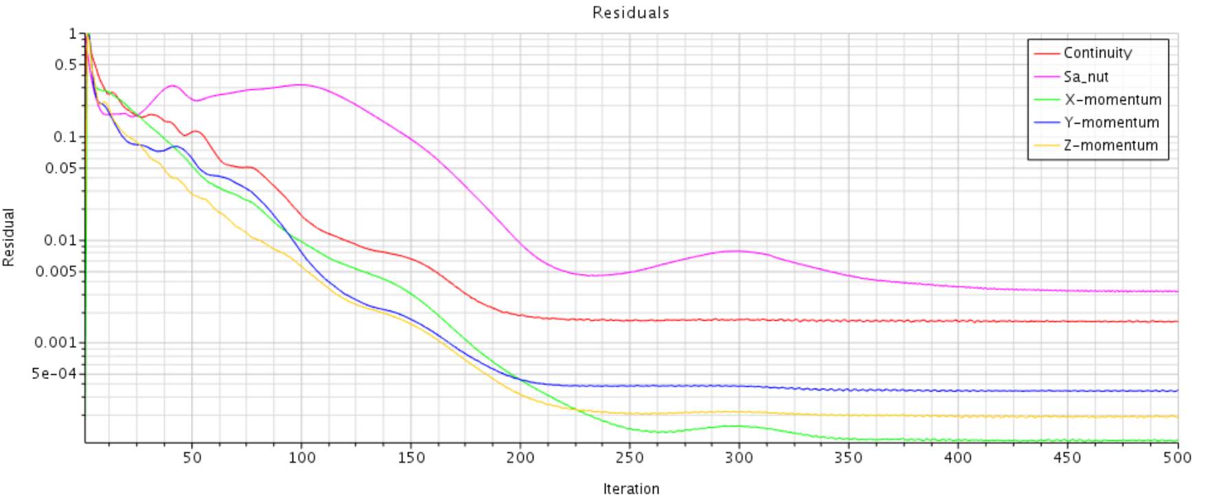
Figure 30 Residual for Clear Iced Wing simulation, AOA of 10
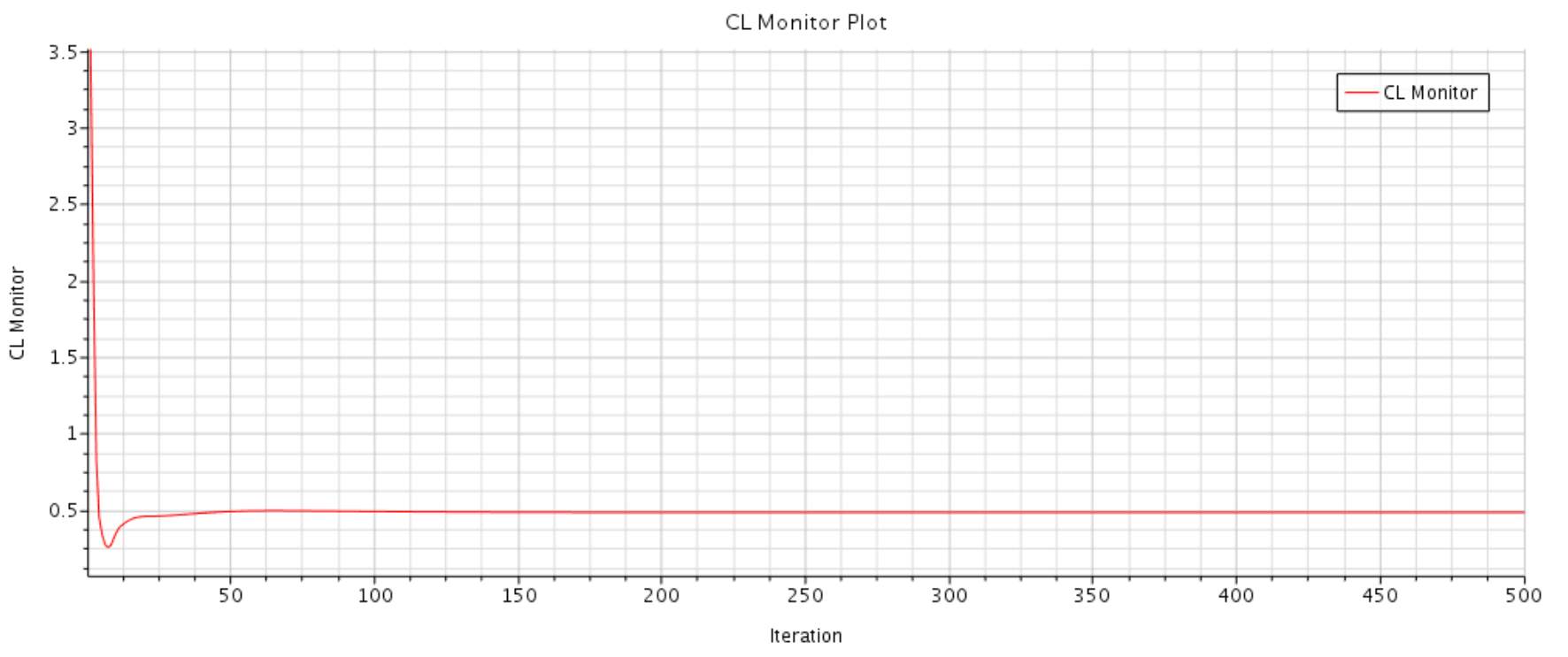
Figure 31 CL Plot for Clear Iced Wing simulation, AOA of 10

Figure 32 CD Plot for Clear Iced Wing simulation, AOA of 10
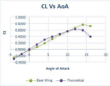
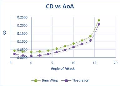 APPENDIX J – THEORETICAL AND EXPERIMENTAL COMPARISON GRAPHS FOR BARE WING
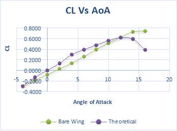
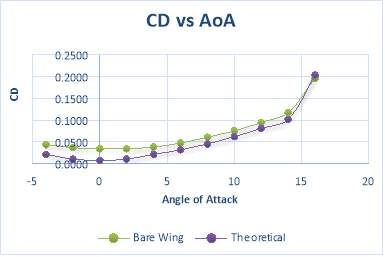
Cite This Work
To export a reference to this article please select a referencing stye below:
Related Services
View all


Related Content
All TagsContent relating to: "Aviation"
Aviation regards any activity involved in the aircraft industry or mechanical flight including flying and the design, manufacture, and maintenance of aircraft. The term “aircraft” includes such vehicles as aeroplanes, helicopters, and lighter than air craft such as hot air balloons and airships.
Related Articles
DMCA / Removal Request
If you are the original writer of this dissertation and no longer wish to have your work published on the UKDiss.com website then please: